1. Introduction

In today’s information-driven society, long-distance signal transmission plays a crucial role in both daily life and military operations. Modulation identification of radio signals is a significant area of research in signal processing, especially in the context of electronic countermeasures in military applications. The challenge of modulation identification in low- and medium-signal-to-noise ratio (SNR) environments is extremely important [1]. Traditional methods, such as maximum likelihood detection, offer superior performance but suffer from exponential complexity, making them computationally expensive and highly dependent on expert knowledge, which limits their widespread adoption [2]. In recent years, deep learning has also been widely used in modulation recognition. Among them, convolutional neural networks (CNNs) have played a crucial role in this field [3]. Additionally, models like residual networks (ResNet) and recurrent neural networks (RNN) have also achieved promising results [4-6]. To further improve model accuracy, various studies have continuously optimized a variety of models. For example, Zhang et al. enhanced the classification ability of CNN and Long Short-Term Memory (LSTM) networks by augmenting the number of input channels to include IQ signals alongside fourth-order cumulants [7]. Lu et al. combined output data from different models to improve their generalization ability [8]. Qi et al. utilized a deep residual network based on ResNet to extract more features, improving the recognition accuracy of multiple modulation schemes, including high-order QAM [9]. However, these models often sacrifice computational efficiency and increase resource consumption in favor of improved accuracy, making them unsuitable for mobile or embedded devices, as well as for applications requiring real-time performance.

To address these challenges and balance computation with accuracy, this paper proposes the use of MobileNetV4, a lightweight neural network architecture. MobileNetV4 leverages depthwise separable convolutions and pointwise expansion to enhance computational efficiency while minimizing information loss. The effectiveness of this approach is demonstrated through evaluation on the public RadioML 2018 dataset.

2. The Architecture Design of Lightweight Neural Networks

This chapter presents the working principles and architecture of the proposed lightweight neural network for signal modulation recognition. The author employs the MobileNetV4-inspired inverted bottleneck structure, which is designed to minimize model size and computational cost. The detailed structure and functions of each layer are explained in this section.

2.1. Inverted Bottleneck Structure

The inverted bottleneck structure is an efficient neural architecture designed to reduce the computational burden while preserving essential information during signal modulation recognition tasks. It usually consists of several key components: a start depth separable convolution, an extended convolution, an intermediate depth separable convolution, a projected convolution, and an end depth separable convolution. In this paper, the end depth separable convolution is not employed.

Traditional convolutions combine channel-wise and spatial information, requiring substantial computational resources. Depth-separable convolution divides this process into two steps—depthwise convolution and pointwise convolution—which significantly reduces computational complexity. This separation ensures that each convolution operation focuses on one aspect of the input, reducing the total number of operations. In standard convolution, each convolution kernel processes all channels of the input feature map simultaneously, fusing the results into the output channels. Suppose the input of the convolutional layer is Win×Hin×Min, where Win and Hin denote the dimensions of the input data and Min denotes the number of input channels, Nout denotes the number of output channels, and the dimensions of the convolutional kernel are denoted as Kw and Kh. The computational and parametric quantities for standard convolution are as follows:

Computational quantity: Win×Hin×Min×Nout×Kw×Kh

Number of parameters: Min×Nout×Kw×Kh

When Min and Nout increase, the computational and data volumes increase rapidly.

In depthwise convolution, spatial convolution is performed separately for each input channel, without fusing channel information. For the input feature map of size Win×Hin×Min, depthwise convolution uses Min independent kernels, each responsible for one input channel. If padding is used, the output feature map has the same dimensions as the input, i.e., Win×Hin×Min. The computational and parametric quantities are as follows:

Computational quantity: Win×Hin×Min×Kw×Kh

Number of parameters: Min×Kw×Kh

Pointwise convolution (using a 1×1 convolution kernel) then combines the channel information and adjusts the number of output channels. For the input feature map Win×Hin×Min, it is processed with N 1×1 convolution kernels, and each convolution kernel processes all the channels. The resulting output feature map is of size Win×Hin×Nout, which satisfies the required number of output channels. In this process, the computational and parametric quantities are as follows:

Calculation amount: Win×Hin×Min×Nout×1×1

Number of parameters: Min×Nout×1×1

Table 1 is a comparison of the computational and parametric quantities of the standard convolution and the depth-separable convolution.

Table 1: Calculated and parametric quantities

Therefore, the calculation is reduced in proportion:

\( \frac{{W_{in}}×{H_{in}}×{M_{in}}×{N_{out}}×{K_{w}}×{K_{h}}}{{W_{in}}×{H_{in}}×{M_{in}}×{K_{w}}×{K_{h}}+{W_{in}}×{H_{in}}×{M_{in}}×{N_{out}}}=\frac{{N_{out}}}{1+\frac{{N_{out}}}{{K_{w}}×{K_{h}}}} \)

The extended convolutional layer usually uses a 1×1 convolutional kernel and serves to increase the number of channels in the input feature map. The required number of channels is determined by the expand_ratio. More channels increases the feature dimensions, enabling the model to capture more information from the input feature map. This extended convolutional layer is usually followed by a depth-separable convolutional layer, which reduces the inflation of the model caused by the increased number of channels and facilitates more efficient feature extraction from the high-dimensional feature map.

In contrast to the dilation convolutional layer, the projection convolutional layer uses a 1×1 convolutional kernel to reduce the dimensionality of the feature map. After expanding the convolutional layer, the number of channels in the model increases significantly. This introduces a significant amount of redundant information while enhancing the feature representation of the model. The projective convolutional layer serves to project the high-dimensional feature maps back into the low-dimensional space, thus removing information that contributes less to the model. This helps control the complexity of the model and prevents overfitting, especially in resource-constrained devices such as mobile or embedded devices. Figure 1 shows the exact composition of an inverted bottleneck structure.

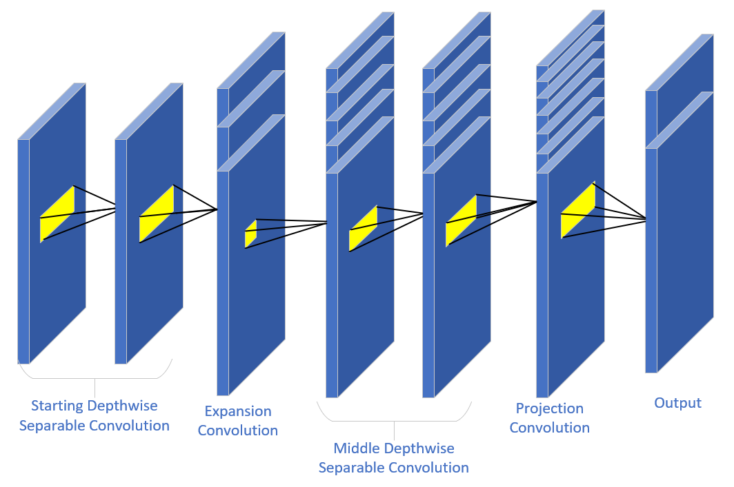
Figure 1: Inverted bottle-neck construction

2.2. Network Structure

The model’s features are initially extracted through a series of convolutional layers. For this experiment, considering the lower computational cost, the first attempt was made to use one-dimensional convolution to extract features. However, after experimentation, it was found that using two-dimensional convolution provided better performance compared to one-dimensional convolution. Table 2 shows the specific composition of the network in this paper.

Table 2: Layer Structure

The loss function used is the cross-entropy loss function, optimized by the Adam optimizer with a learning rate of 0.001. The cross-entropy loss function calculates the discrepency between the predicted probability distribution and the true label distribution (obtained via the softmax function), and the gradient with respect to the parameters of the model is computed. The Adam optimizer adaptively adjusts the learning rate and updates the model parameters according to the calculated gradient. The above process of parameter updating is repeated until the model converges.

3. Experimental Tests and Results

3.1. Dataset and Preprocessing

The data in this experiment uses the open-source dataset RadioML 2018.01A. The dataset contains 'OOK', '4ASK', '8ASK', 'BPSK', 'QPSK', '8PSK', '16PSK', '32PSK', '16APSK', '32APSK', '64APSK', '128APSK', '16QAM', '32QAM', '64QAM', '128QAM', '256QAM', 'AM-SSB-WC', 'AM-SSB-SC', 'AM-DSB-WC', 'AM-DSB-SC', 'FM', 'GMSK', 'OQPSK' 24 types of modulation. The signal-to-noise ratio of each type of modulated signal is in the interval [-20, 30] in 2 dB intervals. For each modulation, there are 4096 data for each signal-to-noise ratio, totaling 2555904 (24 * 26* 4096) data, each of which is IQ data in the format [1024, 2]. The dataset is stored in an HDF5 file where there are 3 parameters: X (IQ signal), Y (modulation mode), and Z (SNR) present. This dataset is large in size, mixes multiple types of higher-order modulations, and takes into account the effects of real-world environment kind of carrier frequency offsets, thermal noise, and so on. In this experiment, the dataset is divided by 6:2:2. The training set is 60% and the validation and test sets are 20% each. Then the X data in the training set, validation set, and test set are adjusted in dimensional order. Reshape the original (batch_size, 1024, 2) to (batch_size, 2, 1024). Extend one dimension on the resized data to finally reshape the X data to (batch_size, 1, 2, 1024). Convert the X and Y data from the training, validation and test sets from numpy.ndarray to torch.Tensor and convert the data type to float and finally transfer the data to the GPU used in this paper. The data is tested at multiple signal-to-noise ratios.

3.2. Experimental Environment

Pytorch version: 2.0.0

Cuda version: 11.8

GPU: NVIDIA GeForce RTX 3090 remotely on the AutoDL platform

Number of GPU: 1

CPU: 14 vCPU Intel(R) Xeon(R) Platinum 8362 CPU

RAM: 45GB

Batch size: 32

Training epochs: 100

Optimizer: Adam lr=0.001, betas=(0.9,0.999), eps=1e-8, weight_decay=0

3.3. Analysis of Results

The control neural networks used in this experiment are CNN1, CNN2 and ResNet [10]. Experiment with these three networks and the lightweight network in this article in the same configuration. The results are shown in Table 3 and Figure 2.

Table 3: Accuracy at different SNRs

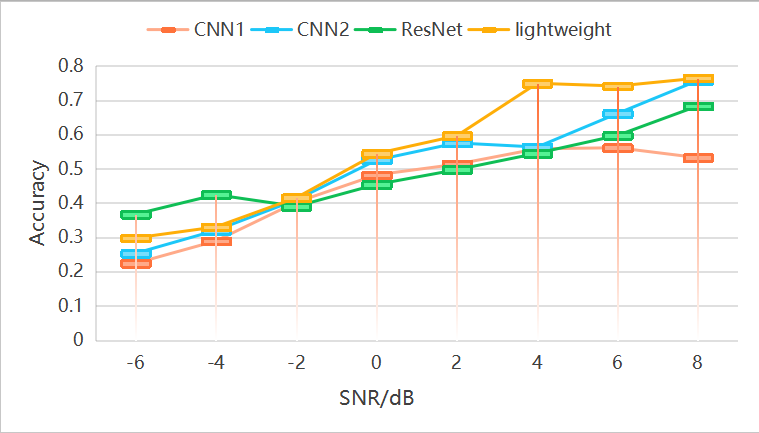
Figure 2: Accuracy at different SNRs

From Table 3, it can seen that the recognition of the neural network in this paper is significantly better than the CNN1 neural network, and compared with CNN2 and ResNet in some signal-to-noise ratio. From Figure 2, we can see that the model in this paper has reached more than seventy percent accuracy at 4 dB, while several other models have a relatively slow rate of accuracy improvement and need to be at 8 dB or even higher SNR to reach 70% accuracy, and it can be seen that the model in this paper performs better at low SNR. In the same experimental environment, the number of parameters of the neural network in this article is 2523416, while the training time per round is 23s, which is 1.22 times that of CNN1 and about 0.4 and 0.36 times that of CNN2 and ResNet. The experimental results show that the neural network in the article has the ability to reduce the size of the model and the computation time while ensuring the correctness of the model.

The following is the confusion matrix of the neural network in this article at partial signal-to-noise ratios.

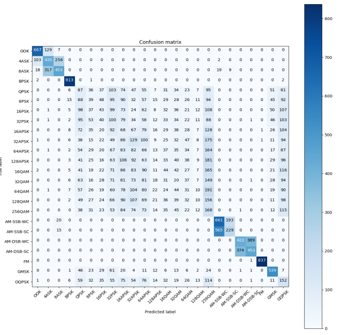
Figure 3: SNR=-4

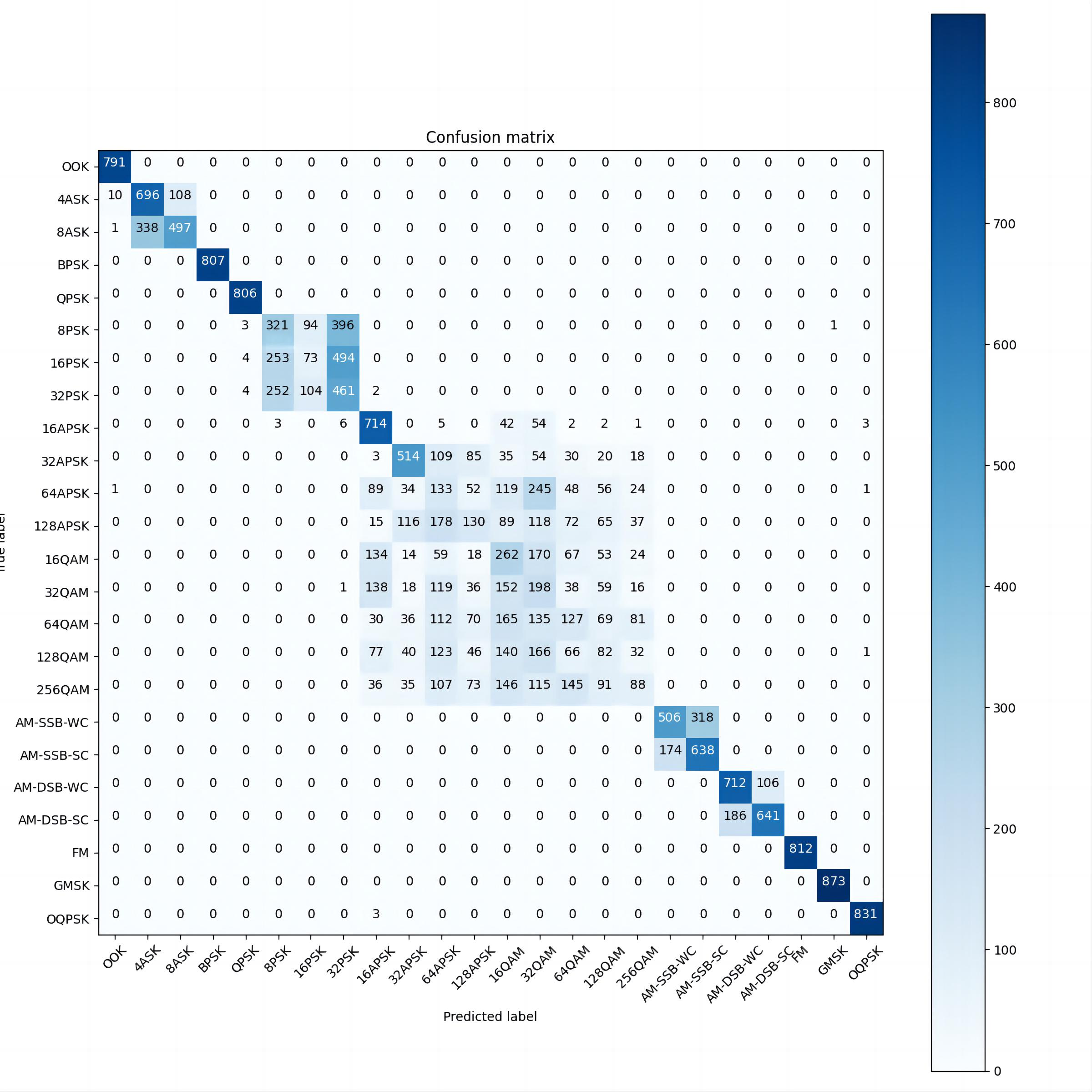
Figure 4: SNR=2

Figure 5: SNR=8

As can be seen from the confusion matrices at different SNRs (Figures 3, 4, and 5), the recognition accuracy of this neural network for low-order modulation modes is improving significantly as the SNR increases.

However, for some higher-order modulation modes, especially QAM modulation, the recognition ability of the model changes slowly with the increase of SNR, which prevents the overall recognition rate from reaching a high value. This experiment found that CNN and ResNet have the same problem. And if the recognition accuracy needs to be further improved, it is difficult to avoid model inflation. From the confusion matrix, it can be found that whether it is the higher-order PSK, APSK, or QAM, most of the errors occurring in the recognition are due to the misclassification in one of the major classes rather than the confusion with other major classes of modulation.

Therefore, is it possible to construct a two-layer stacked network by using this network as a large classification network and then superimposing multiple small classification networks that can effectively extract PSK features, APSK features, and QAM features so as to avoid putting all the feature extraction work in a single network and to reduce the degree of expansion of the model size and computation.

4. Conclusion

This paper addresses the common issue in existing research, where a focus on accuracy often results in excessively large models and long computation times. To mitigate this, a lightweight modulation recognition network is proposed, drawing inspiration from MobileNetV4. The network outperforms CNN and ResNet networks in signal modulation recognition on the publicly available dataset RadioML 2018.01A, especially at low signal-to-noise ratios, while reducing computation time to only 0.36 times that of ResNet. This demonstrates its ability to maintain accuracy while reducing both model size and computation time, making it more effective in military electronic countermeasures with poor signal environments or scenarios with high real-time requirements.

However, several areas still require improvement. First, although the model reduces computation demands compared to models of the same precision, further experiments are needed to determine its practical viability on mobile and embedded devices. Second, optimizing the batch size and fine-tuning the parameters of each layer in the network could potentially enhance performance. However, thi paper is unable to conduct a comprehensive study due to constraints in computational resources and time.

Finally, the model struggles to accurately recognize certain higher-order modulations, especially QAM modulation. In future communications, signals in 6G and higher frequency bands are expected to dominate, with higher-order modulation patterns playing a more critical role. Therefore, future research should focus on improving the ability to recognize higher-order modulation modes as well as controlling the rapid model inflation brought about by the improved recognition ability.

References

[1]. Zhao, Y., Xu, Y. T., Jiang, H., Luo, Y. J., & Wang, Z. W. (2015). Recognition of digital modulation signals based on high-order cumulants. In 2015 International Conference on Wireless Communications and Signal Processing (WCSP) (pp. 1–5). Nanjing, China.
[2]. Wei, W., & Mendel, J. M. (2000). Maximum-likelihood classification for digital amplitude-phase modulations. IEEE Transactions on Communications, 48(2), 189–193.
[3]. O’Shea, T. J., & West, N. (2016). Radio machine learning dataset generation with gnu radio. In Proceedings of the GNU Radio Conference (pp. 69–74).
[4]. O’Shea, T. J., Roy, T., & Clancy, T. C. (2018). Over-the-air deep learning based radio signal classification. IEEE Journal on Selected Topics in Signal Processing, 12(1), 168–179.
[5]. Kumar, Y., Sheoran, M., Jajoo, G. (2020). Automatic modulation classification based on constellation density using deep learning. IEEE Communications Letters, 24(6), 1275–1278.
[6]. Chang, S., Huang, S., Zhang, R. Y. (2022). Multitask learning-based deep neural network for automatic modulation classification. IEEE Internet of Things Journal, 9(3), 2192–2206.
[7]. Hakimi, S., & Hodtani, G. A. (2017). Optimized distributed automatic modulation classification in wireless sensor networks using information theoretic measures. IEEE Sensors Journal, 17(10), 3079–3091.
[8]. Lu, M., Peng, T., Yue, G.(2021). Dual-channel hybrid neural network for modulation recognition. IEEE Access, 9, 76260–76269.
[9]. Qi, P., Zhou, X., Zheng, S. (2021). Automatic modulation classification based on deep residual networks with multimodal information. IEEE Transactions on Cognitive Communications and Networking, 7(1), 21–33.
[10]. Zhang, F., Luo, C., Xu, J., Luo, Y., & Zheng, F.-C. (2022). Deep learning based automatic modulation recognition: Models, datasets, and challenges. Digital Signal Processing, 129, 103650. https://doi.org/10.1016/j.dsp.2022.103650
Cite this article
Wu,Y. (2025). A Lightweight Modulation Recognition Network Based on MobileNetV4. Applied and Computational Engineering,146,43-50.
Data availability
The datasets used and/or analyzed during the current study will be available from the authors upon reasonable request.
Disclaimer/Publisher's Note
The statements, opinions and data contained in all publications are solely those of the individual author(s) and contributor(s) and not of EWA Publishing and/or the editor(s). EWA Publishing and/or the editor(s) disclaim responsibility for any injury to people or property resulting from any ideas, methods, instructions or products referred to in the content.
About volume
Volume title: Proceedings of SEML 2025 Symposium: Machine Learning Theory and Applications
© 2024 by the author(s). Licensee EWA Publishing, Oxford, UK. This article is an open access article distributed under the terms and
conditions of the Creative Commons Attribution (CC BY) license. Authors who
publish this series agree to the following terms:
1. Authors retain copyright and grant the series right of first publication with the work simultaneously licensed under a Creative Commons
Attribution License that allows others to share the work with an acknowledgment of the work's authorship and initial publication in this
series.
2. Authors are able to enter into separate, additional contractual arrangements for the non-exclusive distribution of the series's published
version of the work (e.g., post it to an institutional repository or publish it in a book), with an acknowledgment of its initial
publication in this series.
3. Authors are permitted and encouraged to post their work online (e.g., in institutional repositories or on their website) prior to and
during the submission process, as it can lead to productive exchanges, as well as earlier and greater citation of published work (See
Open access policy for details).