


1. Introduction
In finance, prediction is a key research area, covering stock market trends and derivative pricing. The complexity of financial data characterized by nonlinear relationships, various factors and irrational behaviors, makes accurate forecasting challenging. Despite these difficulties, economists continue to develop methods to improve predictive accuracy and efficiency due to significant investment potential. Traditional time series forecast models such as ARIMA are commonly used. These models provide good fit and reference value in time series processing, with applications even in fields like tourism forecasting[1]. However, their predictive accuracy declines sharply during significant events, and cumulative errors may increase over time. In machine learning, numerous models like linear regression, decision trees, and ensemble methods like random forests have been applied effectively, for example in studies on oil options volatility[2]. These models are more effective at solving multicollinearity issues and complex functional relationships. The swift advancement of deep learning has propelled neural networks to the forefront, leading to the creation of convolutional neural networks (CNN) and recurrent neural networks (RNN), which are used for complex nonlinear predictive tasks, such as options pricing[3]. Moreover, neural networks have a broader range of applications, such as deep neural networks related to the Kyle single-period model[4]. However, due to the overly intricate relationships between variables, these models only uncover correlations within the data, though some scholars are working on methods to interpret them[5]. RNN performs well in fitting data with temporal dependencies because their feedback loops consider both current and past information. However, RNN faces training challenges like the "vanishing gradient problem". To address long-term dependencies and improve training, LSTM networks are introduced. The key innovation in LSTM is incorporating nonlinear, data-related control into RNN units[6]. This is achieved through a gating mechanism, which includes input, output, and forget gates, enabling the network to learn how to retain, transmit, or forget the information[7]. They have been widely applied in NLP[8], image identification and classification[9], etc. In finance, LSTM models are increasingly used, such as in studies on the SSE 500 index[10] and stock market jump detection[11]. In this paper, we study the prediction effect of ARIMI model and LSTM by constructing portfolio. After that, we use the predicted value to calculate the relevant indicators of the portfolio to verify the effect of the portfolio.
2. Methodology
2.1. Data
A portfolio is created with the S \(\&\) P 500 index, gold, and 2-year U.S. Treasury bonds. The inclusion of gold and Treasury bonds is intended to mitigate prediction errors and hedge against stock market volatility by accounting for various market factors. Data from Yahoo Finance cover daily prices from 2000 to 2023 for these assets. The 2-year Treasury data is converted to daily prices using an initial amount of \(__escape_dollar__\) 1,000 and daily yields, while gold and S \(\&\) P 500 data are daily closing prices. These datasets are then weighted and aggregated to compute the portfolio’s daily prices. During data processing, the first step is to remove missing and outlier values. For the ARIMA model, it is crucial to apply differencing to achieve stationarity in the series. For the LSTM model, the steps of standardizing the data, subtracting the mean and dividing by the standard deviation are taken.
2.2. ARIMA model
The ARIMA (AutoRegressive Integrated Moving Average) model is a fundamental tool in time series analysis, designed to address the limitations of traditional regression methods, which often fail to accurately model the dynamic nature of time series data, resulting in significant prediction errors. These errors typically arise from the inability of direct regression to capture complex data structures and error correlations inherent in time series. As that data might not always be stationary, a differencing process is added, culminating in the ARIMA model[12]. The ARIMA model is composed of three primary elements: Autoregression (AR), Differencing (l), and Moving Average (MA). The autoregressive term describes how current values are related to its past values. Differencing is used to make a unsteady time sequence stationary. The moving average component captures the relationship between series values and past forecast errors. Thus, an ARIMA model is typically denoted as ARIMA(p,d,q) and can be written as:
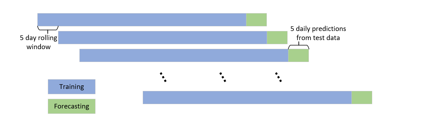
Where \(\Delta^dX_t\) represents the differenced time series after \(d\) operations. We stabilize the data through differencing first, and then select the optimal ARIMA parameters \((p,d,q)\) using the AIC criterion. The ARIMA is the model trained on the first five years of data to forecast the next five days. Using a rolling window approach, we re-fit the ARIMA model for each prediction, generating forecasts for one year, as illustrated in figure 1.
2.3. LSTM
2.3.1. Introduction of LSTM
LSTM networks enhance traditional RNNs by using a memory cell to effectively learn long-term dependencies and address gradient issues. The figure 2 is the process of LSTM,
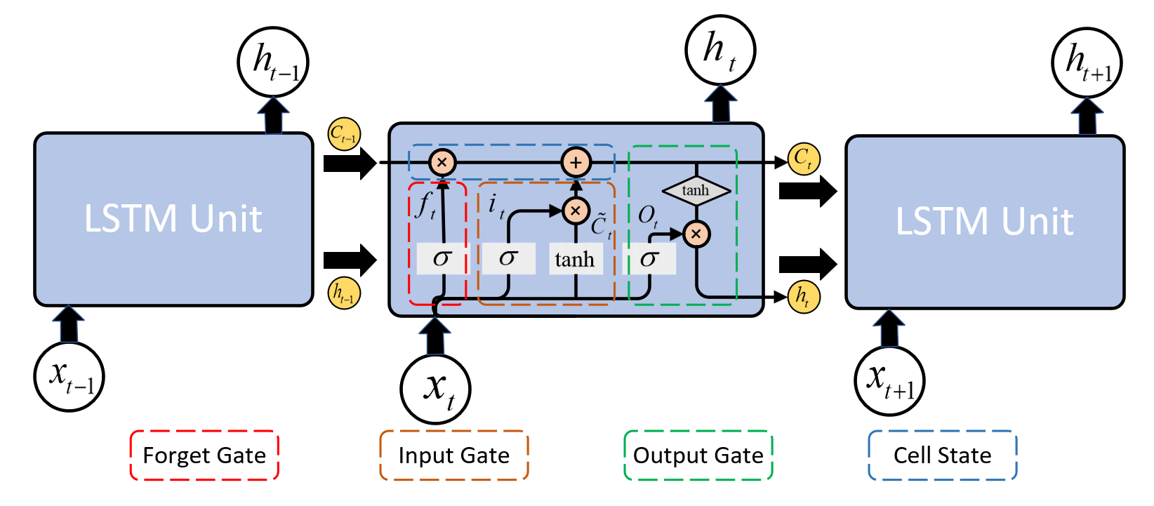
LSTM networks use input, forget, and output gates to manage information flow within the memory cell, effectively balance the intake of new data, retention of past information, and output to enhance modeling of long-term dependencies.
where \(f_{t}\) is the output of forget gate, \(i_{t}\) represents the input gate value, and \(o_{t}\) denotes the output gate activation. And \(\sigma \) is the \(\lt em\gt sigmoid\lt /em\gt \) activation function that make values range between 0 and 1. At time step \( t \) , the cell state \( C_t \) is adjusted by merging the previous cell state \( C_{t-1} \) with the new candidate cell state \( \tilde{C}_t \) , as regulated by the forget gate \( f_t \) and the input gate \( i_t \) . The forget gate determines how much of \( C_{t-1} \) is retained, while the input gate controls the amount of \( \tilde{C}_t \) to be added. The update rule for the cell state is given by,
where \[\tilde{C}_{t} = tanh(W_{C}\cdot[h_{t-1},x_{t}] + b_{C})\] Finally, the output \(h_{t}\) is influenced by both the output gate \(o_{t}\) and the \(\tanh\) function applied to the cell state \(C_{t}\) .
2.3.2. Training and Ensemble
The LSTM model are employed for time series forecasting, using 80 \(%\) of the data for training and 20 \(%\) for testing. The model is trained with a 12-day window size and a batch size of 64, and utilize 96 hidden units to balance complexity and long-term dependency capture. Instead of using a single LSTM network, an ensemble of independently initialized LSTM networks are used. This approach improves prediction, enhances generalization and performance while reducing overfitting. In time series analysis, ensemble LSTM models capture diverse patterns and dependencies, leading to more reliable and accurate predictions. Seven distinct weight initialization strategies are employed to enhance the performance and generalization capability of our LSTM networks. These initialization methods include:
Table 1: Different initializations for each LSTM
| Initialization | Details | Parameters |
| Random Normal | Normal Distribution | \(\mu\) = 0.0, \(\sigma\) = 0.05 |
| Random Uniform | Uniform Distribution | \(\min\) = -0.05, \(\max\) = 0.05 |
| Truncated Normal | Normal Distribution where \(\sigma\) \(\ge\) 2 are redrawn | \(\mu\) = 0.0, \(\sigma\) = 0.05 |
| Xavier Normal | Normal Distribution | \(\mu\) = 0.0, \(\sigma = \sqrt{\frac{2}{fan\_in + fan\_out}}\) |
| Xavier Uniform | Uniform Distribution with [- \(limit\) , \(limit\) ] | \(limit = \sqrt{\frac{6}{fan\_in + fan\_out}}\) |
| Identity | Identity matrix | |
| Orthogonal | Orthogonal matrix |
3. Result
3.1. Result of ARIMA
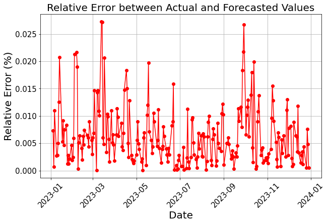
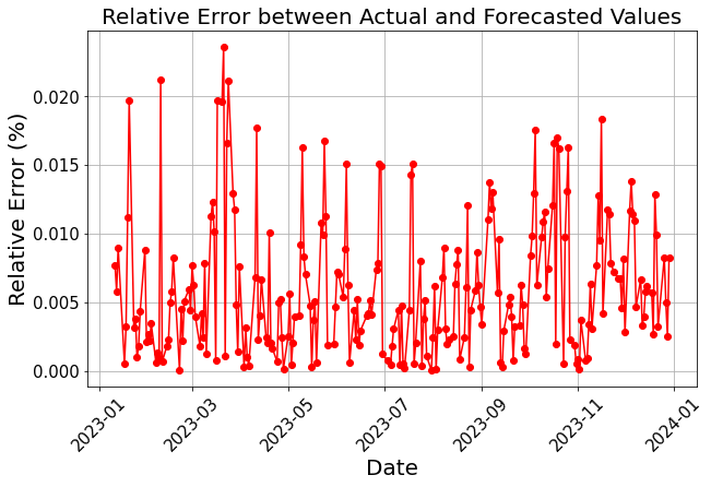
Figure 3 shows the relative error of ARIMA model predictions for portfolio prices with training periods of one year and 2 years. The average relative error is approximately 0.0063 for the 1-year model, and 0.0061 for the 2-year model. There are similar trends about notable errors in March and October 2023 likely due to random or seasonal factors.
 (a) 1-year Training Set
 (b) 2-year Training Set
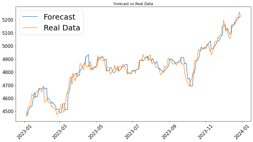
Further observation of the price trends, shown in figures 4 with the same sequence as the relative error plots, reveals that the predicted price trends lag behind the actual data. The predicted volatility is also slightly lower, but the overall trend remains consistent.
 (a) 1-year Training Set
 (b) 2-year Training Set
3.2. Result of LSTM
By using seven different LSTM networks, the prediction figures of some of these distinct initial weight LSTM networks are as followed.
.png) (a) Random Normal
(a) Random Normal
.png) (b) Random Uniform
(b) Random Uniform
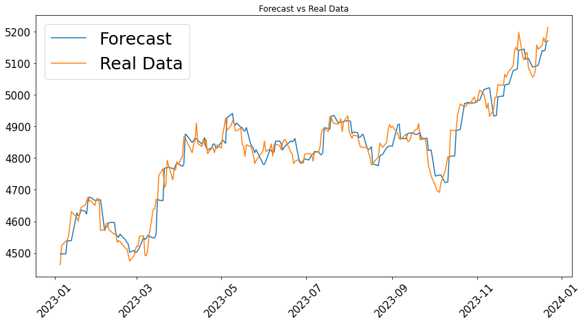
Figure 5 illustrates the predictive performance of the LSTM model by comparing the actual observed data (depicted in blue) with the model's predictions (depicted in red) over time. The close alignment between the model's predictions and the actual values demonstrates the model's effectiveness in capturing overall trends and significant fluctuations. This indicates the successful learning of temporal dependencies inherent in the time series data. Prediction errors are associated with major global disruptions. In early 2022, U.S. inflation prompted aggressive monetary tightening, which heightened market volatility and posed challenges to the LSTM model's predictive accuracy. Additionally, the Russia-Ukraine conflict and the ongoing effects of COVID-19, including supply chain disruptions, further complicated market conditions and predictions. These factors collectively contribute to the observed inaccuracies in the model's forecasts. In the final prediction, the mean value of forecasting outcome of seven LSTM networks are taken with distinct initial weight configuration, and sketch the figure of relative errors as following.
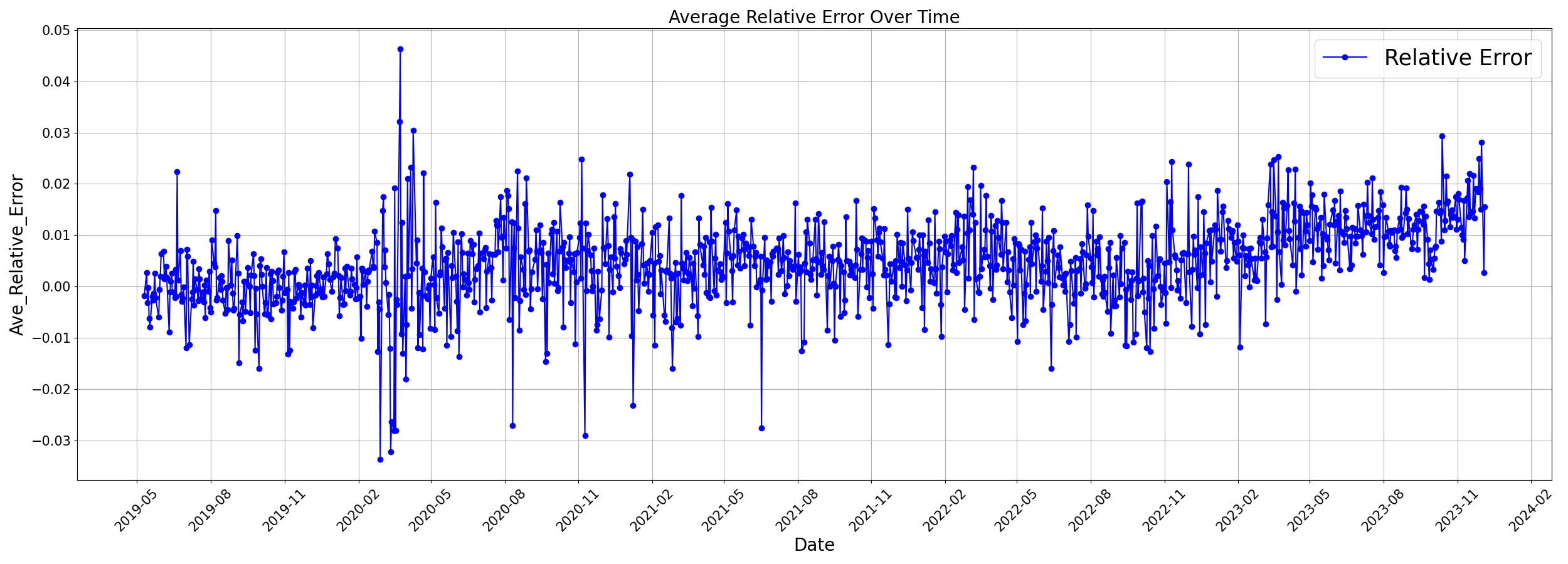
Figure 6 shows the average relative error over time, with a mean of 0.45414 \(%\) . The spikes in early 2020 and early 2022 are attributed to the COVID-19 pandemic and the Russia-Ukraine conflict, resulting in sudden market changes and challenged prediction accuracy. Overall, the model performs well but struggles during major market disruptions.
3.3. Return, Volatility, and Value at Risk (VaR)
Using the LSTM model's predictions, we calculate these indicators.

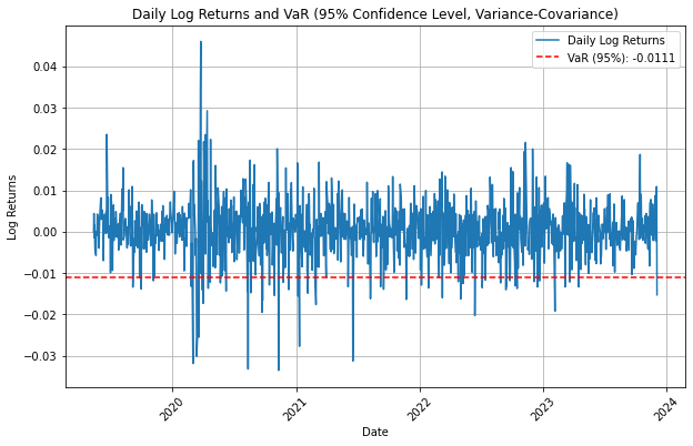
Figure 7 and [???] show that log returns oscillate within a 0.02 range, with notable fluctuations in early 2020 due to the pandemic. Volatility exhibits cyclic patterns characterized by rapid increases followed by periods of stabilization, mirroring market cycles but with varying amplitudes. Post-2020, there is a slight increase in volatility, likely attributed to heightened uncertainty following the pandemic. The VaR value of about -0.01 suggests that with 95 \(%\) confidence, daily returns will exceed this level. It is convinced that data below this threshold is affected by extreme events. The method of variance-covariance is adopted to calculate the value at risk at this point.
4. Conclusion
In conclusion, the use of LSTM networks and ARIMA models to forecast stock prices offers valuable insights for financial time series prediction. The LSTM model excels in its ability to analyze nonlinear relationships and large amounts of historical data which makes them particularly effective for stock price calculations. The strength of the ARIMA model lies in that it can analyze linear relationships with ease which makes them very suitable when analyzing simple markets. In future research, a promising direction is to use the prediction model to optimize and dynamically adjust the portfolio to make our returns higher. In addition, no direct integration of models has not been completed, and integrating multiple models will also be a good research direction.
Acknowledgement
Nan Zheng and Cuiyang Huang made equal contributions to this work and should both be regarded as co-first authors.
References
[1]. Renuka Devi, Alok Agrawal, Joydip Dhar, and A.K. Misra. Forecasting of indian tourism industry using modeling approach. MethodsX, page 102723, 2024.
[2]. Hongwei Zhang, Xinyi Zhao, Wang Gao, and Zibo Niu. The role of higher moments in predicting china’s oil futures volatility: Evidence from machine learning models. Journal of Commodity Markets, 32:100352, 2023.
[3]. Robert Culkin and Sanjiv R. Das. Machine learning in finance: the case of deep learning for option pricing. Journal of Investment Management, 15(4):92–100, 2017.
[4]. Paul Friedrich and Josef Teichmann. Deep investing in kyle’s single period model. arXiv preprint arXiv:2006.13889, 2020.
[5]. Jian-Xun Mi, An-Di Li, and Li-Fang Zhou. Review study of interpretation methods for future interpretable machine learning. IEEE Access, 8:191969–191985, 2020.
[6]. Alex Sherstinsky. Fundamentals of recurrent neural network (rnn) and long short-term memory(lstm) network. Physica D: Nonlinear Phenomena, 404:132306, 2020.
[7]. Carmina Fjellstr¨ om. Long short-term memory neural network for financial time series. In 2022 IEEE International Conference on Big Data (Big Data), pages 3496–3504. IEEE, 2022.
[8]. Wenpeng Yin, Katharina Kann, Mo Yu, and Hinrich Sch¨ utze. Comparative study of cnn and rnn for natural language processing. arXiv preprint arXiv:1702.01923, 2017.
[9]. Jiang Wang, Yi Yang, Junhua Mao, Zhiheng Huang, Chang Huang, and Wei Xu. Cnn-rnn: A unified framework for multi-label image classification. In Proceedings of the IEEE Conference on Computer Vision and Pattern Recognition, pages 2285–2294, 2016.
[10]. Jian Cao, Zhi Li, and Jian Li. Financial time series forecasting model based on ceemdan and lstm. Physica A: Statistical Mechanics and its Applications, 519:127–139, 2019
[11]. Jay F.K. Au Yeung, Zi-Kai Wei, Kit Yan Chan, Henry Y.K. Lau, and Ka-Fai Cedric Yiu. Jump detection in financial time series using machine learning algorithms. Soft Computing, 24:17891801, 2020
[12]. Robert H. Shumway and David S. Stoffer. Arima models. Time Series Analysis and its Applications: With R Examples, pages 75–163, 2017
Cite this article
Zheng,N.;Huang,C.;Dufour,J. (2025). LSTM Networks and ARIMA Models for Financial Time Series Prediction. Applied and Computational Engineering,134,56-63.
Data availability
The datasets used and/or analyzed during the current study will be available from the authors upon reasonable request.
Disclaimer/Publisher's Note
The statements, opinions and data contained in all publications are solely those of the individual author(s) and contributor(s) and not of EWA Publishing and/or the editor(s). EWA Publishing and/or the editor(s) disclaim responsibility for any injury to people or property resulting from any ideas, methods, instructions or products referred to in the content.
About volume
Volume title: Proceedings of the 5th International Conference on Signal Processing and Machine Learning
© 2024 by the author(s). Licensee EWA Publishing, Oxford, UK. This article is an open access article distributed under the terms and
conditions of the Creative Commons Attribution (CC BY) license. Authors who
publish this series agree to the following terms:
1. Authors retain copyright and grant the series right of first publication with the work simultaneously licensed under a Creative Commons
Attribution License that allows others to share the work with an acknowledgment of the work's authorship and initial publication in this
series.
2. Authors are able to enter into separate, additional contractual arrangements for the non-exclusive distribution of the series's published
version of the work (e.g., post it to an institutional repository or publish it in a book), with an acknowledgment of its initial
publication in this series.
3. Authors are permitted and encouraged to post their work online (e.g., in institutional repositories or on their website) prior to and
during the submission process, as it can lead to productive exchanges, as well as earlier and greater citation of published work (See
Open access policy for details).
References
[1]. Renuka Devi, Alok Agrawal, Joydip Dhar, and A.K. Misra. Forecasting of indian tourism industry using modeling approach. MethodsX, page 102723, 2024.
[2]. Hongwei Zhang, Xinyi Zhao, Wang Gao, and Zibo Niu. The role of higher moments in predicting china’s oil futures volatility: Evidence from machine learning models. Journal of Commodity Markets, 32:100352, 2023.
[3]. Robert Culkin and Sanjiv R. Das. Machine learning in finance: the case of deep learning for option pricing. Journal of Investment Management, 15(4):92–100, 2017.
[4]. Paul Friedrich and Josef Teichmann. Deep investing in kyle’s single period model. arXiv preprint arXiv:2006.13889, 2020.
[5]. Jian-Xun Mi, An-Di Li, and Li-Fang Zhou. Review study of interpretation methods for future interpretable machine learning. IEEE Access, 8:191969–191985, 2020.
[6]. Alex Sherstinsky. Fundamentals of recurrent neural network (rnn) and long short-term memory(lstm) network. Physica D: Nonlinear Phenomena, 404:132306, 2020.
[7]. Carmina Fjellstr¨ om. Long short-term memory neural network for financial time series. In 2022 IEEE International Conference on Big Data (Big Data), pages 3496–3504. IEEE, 2022.
[8]. Wenpeng Yin, Katharina Kann, Mo Yu, and Hinrich Sch¨ utze. Comparative study of cnn and rnn for natural language processing. arXiv preprint arXiv:1702.01923, 2017.
[9]. Jiang Wang, Yi Yang, Junhua Mao, Zhiheng Huang, Chang Huang, and Wei Xu. Cnn-rnn: A unified framework for multi-label image classification. In Proceedings of the IEEE Conference on Computer Vision and Pattern Recognition, pages 2285–2294, 2016.
[10]. Jian Cao, Zhi Li, and Jian Li. Financial time series forecasting model based on ceemdan and lstm. Physica A: Statistical Mechanics and its Applications, 519:127–139, 2019
[11]. Jay F.K. Au Yeung, Zi-Kai Wei, Kit Yan Chan, Henry Y.K. Lau, and Ka-Fai Cedric Yiu. Jump detection in financial time series using machine learning algorithms. Soft Computing, 24:17891801, 2020
[12]. Robert H. Shumway and David S. Stoffer. Arima models. Time Series Analysis and its Applications: With R Examples, pages 75–163, 2017