1. Introduction

This paper concludes with some hybrid methods to solve this problem and provides different ways to generate the potential field. We also give some different perceptions of how to analyze the Potential Field.

In Hagelba¨ck’s method [1], we will give more details about calculating the potential field and show how to use it in some simple RTS games. We will solve the dead ends and narrow passage problem. Then, we will show how to build a potential field, set an ultimate target, and use it for navigation and making decisions. However, the original Potential Field is influenced by the local optima. The author let the units randomly walk in this paper to solve the local optima problem. In [2], a hybrid navigation algorithm is introduced, utilizing A* when there are no enemy units or buildings in sight and switching to potential fields during combat. This method addresses the issue of local optima that can occur with potential fields—where units might become trapped in intricate terrain—by employing A* while also leveraging the advantages of potential fields for unit positioning in battle scenarios.

In [3], while potential field methods are adaptable, they often encounter local minima issues. This paper proposes a hybrid approach combining flow fields with the A* algorithm, improving path planning efficiency and overcoming common pitfalls in complex environments.

We think it would be interesting to find methods to improve this algorithm. We found three papers that discuss the Artificial Potential Field. In fact, there are also many problems in the Artificial Potential Field, so we can hardly use one way to find the path. Instead, the papers develop a hybrid method to solve the problems in the Artificial Potential Field. They use a Potential Field with A* to solve problems like local optima or some pre-calculated information to reduce the algorithm’s time to use it. Another problem is that we need to check if there are some dead ends and narrow passages to improve the algorithm.

We think it’s an interesting algorithm for solving problems in robotics and games, especially real-time strategy games. As it’s a very efficient algorithm used in multi-agent systems, we want to introduce modern usage to research.

2. Background

Finding a path is important for many things, so many algorithms have come up to solve this problem. For many years, game developers have used algorithms like A* to solve path-finding. However, only a few papers focus on the Potential Field algorithm. A universal idea of an algorithm like A* is to speed up a single unit to find the path. However, the Potential Field uses the terrain information, other units’ status, and the high-level target to find the path. The algorithm can speed up all the units to find paths together by handling all this information. Compared with other algorithms that handle the needs individually, the Potential Field can handle all the needs simultaneously. However, since 1985, Ossama Khatib introduced the Potential Field in [4], the algorithm has hardly been used in game development.

Potential Field path planning computes the potential at each node within an environment, enabling multiple agents to navigate the space without the need to calculate individual paths for each agent. This method allows agents to move efficiently while avoiding obstacles and other agents by following the gradient of the potential field. The algorithm builds the Potential Field by calculating the potential of each tile. The potential Field algorithm can get the map’s potential and then the field’s speed vector. The speed vector is the direction and the speed at which the agent should go on specific tiles. Then, the algorithm assigns the speed vector to the agents. The units go to the tiles that have the highest potential around them.

Real-time strategy (RTS) games present significant challenges for AI bot developers. Players typically begin with a central base and a group of workers. These workers are responsible for collecting various types of resources, which are then used to build structures. These structures play crucial roles in expanding the base, defending it, and producing combat units. Additionally, RTS games often feature technology trees, allowing players to invest resources into upgrading units and buildings. Players must make numerous strategic decisions about resource allocation, as resources are finite and require accumulating time. For instance, resources can be allocated to produce inexpensive units for an early offensive (commonly known as a rush tactic), to construct strong defenses with immobile turrets and bunkers, or to advance technology for powerful units, which may leave the player exposed in the early stages of the game.

3. Artificial Potential Field in RTS Game to Making Decisions

In Hagelba¨ck’s Algorithm [1], an experimental framework based on the Artificial Potential Field was employed to make RTS games, including finding paths and making decisions. The experiment is conducted on Open Real-time Strategy (ORTS), a real-time strategy game designed as a platform for users to test artificial intelligence (AI), particularly for game AI applications.

This method has six phases.

The first phase is classifying objects. The algorithm needs to understand the different kinds of obstacles in the game, such as static terrain and moving units, and what objects remain in attention throughout the scenario’s lifetime.

The second phase is classifying the driving forces of different targets, where the algorithm identifies the game’s driving forces relatively abstractly, such as avoiding obstacles and attacking opponent units. Calculating different driving forces fields requires the algorithm to save multiple fields to isolate certain aspects of the potential computation. Additionally, the algorithm can give them a dynamic weight separately. The third phase is assigning charges to the objects. The algorithm needs to calculate all the potential fields and then add them up. However, some fields, like static terrain fields of navigation, can be pre-calculated to save CPU time.

The fourth phase is deciding the granularity of time and space. The algorithm needs to handle time and space. If an agent needs to move around the environment, both measure the impact on the future. So, the algorithm needs to calculate how far the unit can go, and the time determines how far the unit may move in one frame.

The fifth phase is building a single agent. The algorithm must let each agent know what the other agents are doing. Then, it needs to calculate the possible behavior. It may use a heuristic function to calculate the potential in an individual field.

The sixth phase is the collaboration of multiple agents, where the algorithm designs an architecture of the multiple agents. Here, it takes the unit agents identified in the fifth phase. It may give them specific missions and roles or add the additional information (possibly) needed for coordination.

3.1. Methodology

1. Classifying objects: In Hagelba¨ck’s method [1], they identify the objects: Cliffs, Sheep, and own (and opponent) tanks, marines, and base stations. This depends on the specific situation.

2. Building fields: In Hagelba¨ck’s algorithm [1], there are three driving forces in ORTS:

(1). Avoid colliding with moving objects and cliffs

(2). Hunt down the enemy’s force

(3). Defend the bases

The algorithm needs to compute three distinct fields: the navigation, strategic, and tactical fields. The navigation field is created based on static terrain, providing agents with information about passable and impassable areas. The strategic field assesses the overall layout and positions of units and objectives, while the tactical field focuses on immediate environmental threats and opportunities. Together, these fields guide agents in their decision-making processes. The strategic field is an attracting field; it makes units move toward the opponent’s objects. The tactical field can help schedule all units.

3. Assigning charges: Each object in the environment, such as cliffs, sheep, or units, has a set of charges that generate a potential field around it. These fields influence the surrounding space, with each object contributing based on its properties. The fields generated by all objects are weighted and combined to form a total potential field. Agents use this combined field to guide their decision-making and action selection, moving based on the highest or lowest potentials within the field. The total field directs agents by influencing their movement towards goals and away from obstacles based on the combined potential values. The actual formulas for calculating the potential fields depend greatly on the application. Here are some examples used in the experiment.

a) Cliff: The cliff generated a repelling field of obstacle avoidance. The potential \( {p_{cliff}}(d) \) at a distance d (in tiles) from a cliff is a negative number when the distance is zero and decreases as the distance increases. Here, the “decreases” means it gets more negative. An example is the equation below:

\( {p_{cliff}}(d)=\begin{cases} \begin{array}{c} -80/{d^{2}} if d \gt 0 \\ -80 if d≥0 \end{array} \end{cases} \) (1)

When multiple cliffs influence a tile, it takes the minimum potential.

After calculating all the potential fields generated by static terrain, the navigation fields are post-processed in two steps to improve the agents’ abilities to move in narrow passages and avoid dead ends.

1) The algorithm checks if cliffs are in all 16 directions within five tiles. If there are more than nine directions that have cliffs, it considers the tile (x, y) as a dead end, and a sample is like Fig 1.

2) The algorithm handles a narrow passage between cliffs by checking if a tile (x, y) meets one of the following conditions: a sample is like Fig 2

Figure 1: The figure is an example in article [1]. White tiles represent passable areas, black tiles denote impassable areas, and grey tiles indicate sections filled in by the algorithm to eliminate dead ends.

a) the tile (x + 1, y) has negative potential and the tile (x1, y) has negative potential.

b) the tile (x, y + 1) has negative potential and the tile (x, y − 1) has negative potential.

if any condition is met, the potential of (x, y) is set to 0.

Figure 2: Example of the narrow passage in article [1]. White tiles have a potential of 0; the darker the color, the more negative potential a tile has.

b) The opponent units: When considering the opponent units, the algorithm keeps them within the Maximum Shooting Distance (MSD). So, the ring whose radius is MSD has the maximum potential, which is greater than 0. If our units are too far from the opponent units, such as outside the Maximum Detection Range (MDR), the potential is 0.

c) Own bases: Bases generate a repelling field for obstacle avoidance. The base is similar to a static obstacle. But note that if the bases are bigger, the farthest distance is the diagonal of the base, so there is a bit of difference from the static terrain. It generates negative potential when the tiles are near our bases and is zero if they are too far from them.

d) The own units and sheep: Own units and sheep are all moving obstacles for a specific agent, so their potential function is similar. They generate a repelling field for obstacle avoidance, too. At the same time, the potential is zero if the tiles are far from them, and if they become near them, the potential is negative.

4. Decide the granularity: The game map is \( 1024×1024 \) , and the terrain is constructed from tiles of \( 16×16 \) . The paper [1] uses \( 8×8 \) to construct our potential field to get more details for deciding. However, the side effect is that it needs more memory and time to calculate the potential field. In this experiment, \( 8×8 \) is enough to handle everything within the proper time and memory.

5. The unit agent: Let each agent make decisions with the tiles that have the maximum potential. If a unit can attack an opponent unit, it attacks it. Otherwise, the unit moves to the tile with the maximum potential around it.

After making a decision, let other units know. Because the movement will change the potential in the future, the algorithm needs to calculate the movement’s influence. Then, other units can avoid collision with the units. So, the tactical field must be updated to change others’ decisions. If an agent has been idle for some time, let it randomly move in a direction to get out of local optima. If an opponent unit is within the maximum shooting distance, attack the opponent unit.

For example, if units A and B want to move to a tile (x, y). If unit A updates first, B can avoid collision with unit A. The unit B will go to another tile.

When the unit attacks an opponent unit, the unit must consider avoiding obstacles while keeping the opponent unit within the maximum shooting distance. In this situation, the units themselves can also be considered obstacles.

6. The multi-agent system: In different games, there may be different tactical targets. So, sometimes, people can set high- level targets.

3.2. The experiment

1. Environment: Two different games were used in the experiment.

(1) In Tank Battle, each player controls multiple tanks and several bases. For this experiment, each player has50 tanks and five bases. The tanks have long-range, powerful fire capabilities but a long cool-down period. The cool-down period means the time between shots. Bases are highly durable and can absorb significant damage before destruction but cannot attack other units. The game’s map features randomly generated terrain, which includes passable lowland areas and impassable cliffs, adding complexity to movement and strategy.

(2) In Tactical Combat, each player controls a group of marines, with the objective being to eliminate all opposing marines. In this experiment, each player has 50 marines. The Marines can fire rapidly and possess average firepower. At the start of the game, they are randomly positioned on either the right or left side of the map. The map consists of passable lowland terrain, allowing unrestricted movement across the battlefield.

2. Result: In the experiment, the algorithm won more than one-third of the teams in the tank battle game shown in Table 1 and won at least one second of teams in the tactical games shown in Table 2.

WarsawA maps each unit’s position to a node on a grid to determine optimal paths. They target the enemy along a line, focusing on its weakest points at a specified range.

WarsawB utilizes a dynamic graph with moving objects to find paths. While their units repel one another, they remain grouped in a large squad. During an attack, they spread out along a line at MSD, with each unit targeting the weakest enemy within range. In tactical combat, each unit aims to align with the same y-coordinate as its designated enemy target.

Table 1: Summary of the results of Orts tank-battle 2007 in the article [1]

Table 2: Summary of the results of the orts tactical combat in the article [1]

Uofa employs a hierarchical command system, including roles like squad commanders and path-finding commanders, to organize and control units. The units are grouped into clusters and attempt to encircle enemy forces by spreading to MSD.

Umich adopts a strategy driven by finite-state machines, guiding the overall tactics. For instance, units are organized into a single squad focused on hunting enemies, primarily emphasizing attacking opponent bases as their top priority.

Umaas and Uofa entered the competition with their 2006 entries. No entry descriptions are available, and how they work is unknown.

3. Discussion: The experiment shows that the artificial potential field is a good fit for solving real-time strategy game problems compared to other algorithms. A PF-based solution may replace path planning with a heuristic method if the analysis is carried out carefully but efficiently [1]. Potential Field gives us an efficient and flexible method to solve the problem of finding paths and making decisions with multiple agents. But there are still some disadvantages:

• The first issue pertains to resolution in the algorithm. The agent currently moves to the center of the 8x8 grid tile with the highest potential. This approach fails when the agent encounters nearby units or needs to navigate narrow passages. A potential solution is to enhance the functionality to estimate potential at a more granular point level, allowing for finer movement. Increasing the map resolution could improve navigation, though this approach is computationally expensive.

• The Second issue is that the algorithm can’t correctly find the weakest opponents. Sometimes, it attacks a very difficult field to break because it is a local optima. In other words, the Potential Field method focuses on the local optima and is always misled by it.

More experiments are needed to improve the algorithm or find different ways to optimize the parameters. This is a field worth researching.

4. Potential-Field-Based Navigation in Starcraft

Real-Time Strategy (RTS) games, a sub-genre of strategy games, are typically set in a war environment and present significant challenges for both AI and human players. Traditional pathfinding algorithms like A* often fall short in dynamic game environments due to their static nature. In [2], a novel navigation algorithm based on potential fields is introduced, which combines A* with potential fields to address the dynamic elements of RTS games more effectively.

4.1. Challenges

In RTS games, armies typically consist of numerous units that need to navigate the game environment effectively. The real-time and dynamic nature of RTS games makes pathfinding a particularly demanding task for AI. The following are key challenges faced in RTS pathfinding:

1. Dynamic and real-time aspects of RTS games: The constantly changing and real-time nature of RTS games presents significant difficulties for pathfinding. Traditional algorithms like A* struggle to handle these dynamic environments without modification [5]. If a movable object obstructs the path, having been located elsewhere during the initial calculation, the route is rendered invalid, requiring the agent to recalculate all or part of it.

2. The problem of local optima: Another problem of potential fields is the risk of the agent becoming trapped in a local optimum, where the current position has the highest potential but is not the desired destination. Figure 3 provides an example of a map that poses significant challenges for a purely potential field-based approach. The top section of the map is displayed in the screenshot, highlighting the starting position of one player, with the other player’s starting position located below. The yellow circle indicates the only entry and exit point for the starting area. If the agents are instructed to move towards the original position of the opponent, the highest potential would lead them south of their own starting position, causing them to overlook the northern exit.

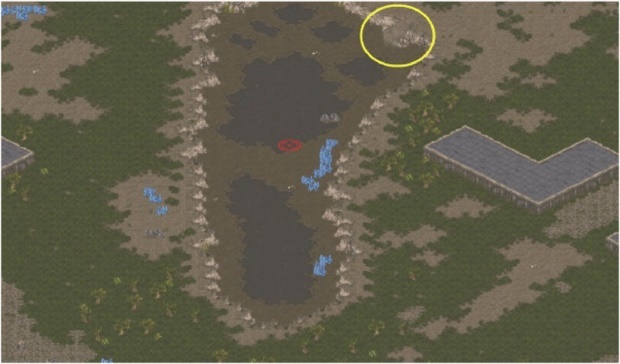
Figure 3: Screenshot from the Baby Step map in the Broodwar expansion. The yellow circle shows the only entry/exit point of the starting area [2].

3. Complex situations: Typically, the total potential field is computed as a weighted sum of all subfields, so a different issue can arise, increasing potential risks in navigation in complex situations. In scenarios where multiple enemy units are concentrated in one area, which is common in RTS games, the highest potential might be centered within the enemy force, leading our agents to mistakenly move towards the opponent’s strongest position [2], as is shown in the upper image in Figure 4.

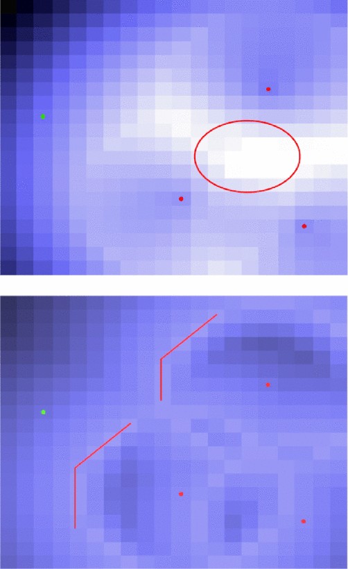
Figure 4: Total potential field when using the sum of opponent fields (left) or the max of opponent fields (right). Light areas have higher potential than darker areas [2].

4.2. Methods

In [2], a hybrid approach combining potential fields and A* is proposed to 1) reduce the occurrence of multiple local optima in potential fields by employing A* where suitable and 2) leverage the dynamic world-handling capabilities of potential fields. In this integrated method, A* is utilized for navigation when the agent detects no enemy units, ensuring efficient pathfinding over long distances. When detecting an enemy unit or structure, the navigation shifts to potential fields, thereby minimizing local optima while taking advantage of the benefits that potential fields offer, such as the ability to surround enemy units.

To mitigate the issue of local optima, the potential field navigation system employs a pheromone-inspired approach.

The total potential field is designed to prevent the most appealing points from being located at the center of enemy formations. This calculation accounts for all relevant objects, excluding enemy units and structures. The proposed solution calculates the overall potential field by taking the maximum value of all potential fields generated by enemy units and buildings rather than using a weighted sum, as is shown in the bottom image of Figure 4. This greatly improved the performance of the ORTS bot.

Another enhancement proposed is to have the generated fields be determined not only by the agent and the object it interacts with but also by the agent’s internal state [2]. The agent is in an attack state, as is presented in the top image of Figure 5, and the potential field created by the enemy unit shows the highest potential at the agent’s maximum shooting distance. Conversely, if the agent is in a retreat state, as is showcased in the bottom image of Figure 5, the highest potential shifts to be outside the opponent’s maximum shooting distance.

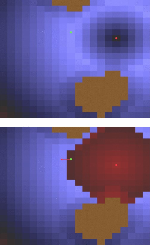
Figure 5: Total potential field for an agent in attack state (left) and in retreat state (right). Red areas are repelling [2].

4.3. Experiments

A series of experiments were carried out to evaluate two versions of a bot navigating the game StarCraft as Terran, each competing with the built-in AI opponents: Terran, Zerg, and Protoss. The first bot version employed only the A* algorithm for navigation, while the second combined A* with a potential field approach. Each bot version played two matches on two different maps against each of the three races.

The chosen maps were:

• Fading Realm: A two-player map distinguished by its multiple plateaus, each set at different heights.

• Destination 1.1: A map designed for two players, prominently showcased in the AIIDE 2011 StarCraft bot competition.

In the first experiment, each bot was faced with built-in AI opponents: Terran, Protoss, and Zerg. The experiment indicated that the built-in AI posed a minimal challenge to both bot versions. Both won 11 out of 12 games, each losing only one game to an early Zealot rush by Protoss. The distinction in their average scores was negligible.

To conduct a more rigorous comparison, a second experiment was performed where the two bot versions competed directly against each other. As is showcased in Table 3, the results revealed that the hybrid A* and potential fields approach was superior, securing 5 out of 6 victories. Importantly, both versions utilized identical strategies, build orders, and squad setups—the sole difference being the use of potential fields when engaging enemy units or structures.

Additionally, games were played using only potential fields for navigation. However, these matches invariably ended in a draw. While the bot demonstrated strong defensive capabilities, it struggled with the complex choke points on the maps. Despite employing a trail containing 20 positions to navigate local optima, the bot couldn’t master sufficient forces to breach enemy defenses and secure a win. This suggests that a more robust method for handling local optima would be necessary for this approach to succeed on typical StarCraft maps.

However, there are still drawbacks in the experiments. As the complexity of maps increases in highly dynamic game environments, more experiments should be carried out to compare the hybrid pathfinding system to a nonhybrid pathfinding system in terms of win ratio in more complex game environments. For example, a noticeable distinction exists between straightforward two-player maps and the more intricate four-player maps, which can lead to significant variations in the outcomes of hybrid and nonhybrid pathfinding for the latter. Plus, more experiments should be performed to test how much hardware resources each of them requires to evaluate their performance better, and there should be more tests for statistical significance, such as a two-sample T-test between proportions. Hence, more improvements can be made to the experiments.

4.4. Discussions

The findings from the two experiments demonstrate that a navigation system combining A* with potential fields surpasses the performance of a bot relying solely on A* for navigation. As previously discussed in this paper, navigation methods based on potential fields are effective at encircling opponents by employing exponential subfields or piecewise linear. However, when integrating potential fields with A*, timing is critical; switching to potential fields too late prevents agents from adequately spreading out around the enemy while switching too early increases the risk of getting trapped in complex local optima.

Table 3: Results from the bot playing against itself.[2]

On the other hand, a navigation system that relied exclusively on potential fields proved ineffective due to the complexity and the numerous local optima present in the chosen StarCraft maps.

5. Real Time Path Planning Using Flow Field and A*

In [3], Path planning refers to the process of identifying a series of configurations without collisions from the starting position to the destination. Several techniques have been introduced, including roadmap methods, visibility graphs, and potential field-based techniques, which consider agents as points within a configuration space influenced by artificial potential fields. Although these techniques can be effective, they are often prone to local minima, where the robot may become trapped due to the A* potential function focusing solely on nearby obstacles [6]. To fix this issue, a better version of the A* algorithm is used, which adds obstacle potential fields to make sure the path is efficient. A* combines the cost of moving to a point with a guess of how far the goal is, often using the Euclidean distance. This method, which can be both optimal and complete in certain situations, is called the Valley Field.

5.1. A. Methodology

1. Problem Formulation: In [3], This paper imagines an agent operating in an unknown area with barriers. In such an area, where there are both passable and impassable regions, an obstacle map can be made using either a node-based system or a grid-based system.

Fig.6 demonstrates an example of a grid-structured environment, where black pixels show barrier nodes and white pixels show nodes without obstacles. Fig.7 is based on this obstacle environment. The obstacle potential field and the target potential field can be created independently.

Obstacle Potential Field: The first step is to combine the potential field of the obstacle. This step uses a modified version of Dijkstra’s shortest route algorithm, applied to each point marked as a barrier. Normally, Dijkstra’s algorithm determines the shortest route from the starting node by building a set of nodes with the minimum distance from the starting point. However, in this version, it doesn’t search for a path; instead, it sets the potential energy while building the obstacle environment. The obstacle potential field creates lower potential energy at the nodes furthest from the obstacle. This part of the algorithm only needs to run once for each unique obstacle environment.

Figure 6: A predefined barrier environment.[3]

2. Target Potential Field: The second step of the algorithm is to calculate the target potential field, starting from the target node. It uses a modified version of a Dijkstra-like shortest path algorithm. In this step, the blue asterisk shows the node with the lowest potential, which is the target node. Nodes that are further from the target are given a higher potential.

Figure 7: Potential field Process [3]

3. Combining Potential Field: The total potential field used in this method is a weighted sum of the obstacle potential field and the target potential field. Therefore, for every node in the grid, the cumulative potential function is calculated as

\( {p_{co}}={k_{1}}*{p_{ob}}+{k_{2}}*{p_{ta}} \) (2)

In this context, \( {p_{co}} \) , \( {p_{ob}} \) , and \( {p_{ta}} \) represent the combined potential, obstacle or barrier potential, and target potential, respectively. The weighted values k1 and k2 influence the path-finding agent operations moving through the environment. Increasing k₁ compared to k₂ will cause agents to avoid obstacles more, as it amplifies the influence of the obstacle potential field.

5.2. B. Result and Discussion

In some situations, the potential change in the combined potential field is zero. This happens in areas where the obstacle’s potential field change cancels out equally with the target’s potential field change. The potential field is depicted in Fig. 8 and Fig. 9.

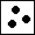
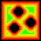
Figure 8: Environment of obstacle [3] Figure 9: The Potential Field of obstacle [3]

As explained in section A, a combined potential field can be created in the given environment. Figure 10 shows how the combined potential field is utilized for guiding agent steering. The star symbols indicate the target nodes that decide the direction of movement.

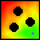
Figure 10: Final Flow Field [3]

This scenario creates an area with constant potential, which could lead to steering problems. This region is more clearly visible in Figure 11, where the potential field vectors (represented by arrows) indicate the direction of potential variation. The area with no change in potential is in the blue rectangle, and a zoomed-in view of this area is shown in Figure 12. In this region, there is no potential differential, resulting in a zero vector.

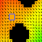
Figure 11: Flow field with the potential field vectors shown as black arrows [3]

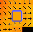
Figure 12: Zoomed in view to visualize the region of zero potential field [3]

This paper provides an alternative strategy for solving the local minimum problem by utilising an improved A* search algorithm based on an obstacle potential field derived from a predictable path. This approach cancels the goal potential field and the combined potential field in favour of the A* routing algorithm. As a result, the A* part of the navigation strategy must be executed individually for each goal and each agent rather than only once per goal.

The A* version of Valley Field Path Planning offers configurability, with key parameters including the smallest separation distance \( {g_{min}} \) and the desired distance from obstacles \( {d_{pref}} \) . Representing the barrier potential of each node is assigned the z-value for the matching 2D position helps to perform the A* search algorithm in conjunction with the barrier potential field. This actually introduces a third dimension that must be considered in the A* search algorithm. Conceptually, we can imagine obstacle nodes as mountain maximum and minimum potential areas as valleys. However, the optimal route planning behavior is not equivalent to navigating through mountainous terrain using A*. The inclination of this terrain is critical in determining the final A* path. If the incline is shallow, A* may opt for a shorter path by traversing over the mountain rather than circumnavigating it. In a 2D environment, this situation would result in the agent closely staying close to obstacles. To prevent this, the slope of the mountain (denoted as k₁) must exceed the maximum possible path length within the environment, particularly in an n × n grid environment.

\( {k_{1}}≥{n^{2}}/2 \) (3)

The meaning of this equation is the highest attainable potential, \( {p_{high}} \) , within an n × n environment, it will be

\( {p_{high}}={k_{1}}*\sqrt[]{{2n^{2}}} \) (4)

The value of k₁ calculated from equation 2 ensures that the agent will navigate through regions of low potential whenever possible. However, if the agent needs to cross a gap containing a zone of elevated potential, it will continue to follow the region of high potential throughout the rest of its route. This occurs because the descent into the valley is longer than all paths around the mountain as a result of the value of k₁. Thus, if the path involves nodes with high potential, the agent will tend to approach the obstacle. The effect of this may be seen in Fig. 13.

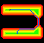
Figure 13: Path (in blue) riding high potential [3]

To avoid this path-planning behaviour, paths moving toward lower potentials must be associated with shorter paths in the A* algorithm. This can be done by reducing the g-cost when ∆p_o < 0. In this scenario, the g-cost represents a function of potential energy. In order to comply with the energy preservation, the total energy gained in moving down to the low potential energy region must equal the energy lost in moving up to the high potential energy region. In addition, the estimated cost function will be evaluated using the same method. With this adjustment to the A* algorithm, routes will be created through low-potential regions, as shown in Figure 14.

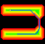
Figure 14: Path (in blue) favoring low potential regions [3]

During the last iteration of the A* version of Valley Field Path Planning, it becomes straightforward to select a preferred obstacle close distance \( {d_{pref}} \) This parameter can be implemented by increasing the baseline of the barrier potential field to match the minimum barrier potential. This minimum potential value, \( {p_{min}} \) , is defined as follows:

\( {p_{min}}={p_{max}}-{k_{1}}*{d_{pref}} \) (5)

In this context, \( {p_{max}} \) represents the maximum potential observed within the obstacle potential field. Beyond the \( {d_{pref}} \) parameter, a minimal gap distance for the path \( {g_{min}} \) can also be readily enforced. This is accomplished by designating any node with an obstacle potential exceeding \( {p_{gap}} \) as non-navigable. The gap potential, \( {p_{gap}} \) , can be determined using equation 4.

The A* modification of Valley Field Path Planning provides a cost-effective solution for configurable through-wall distances and minimum gap widths. Both methods can be extended to three dimensions. In the A* variant, the obstacle potential field introduces a fourth dimension.

6. Conclusion

Our research highlights several important advantages of artificial potential fields (APFs), including their ability to manage multiple agents simultaneously and their adaptability to dynamic gaming environments. However, challenges such as local minimums and computational complexity remain, so there is an A* need to integrate A* algorithms to address these limitations by combining improved A* Algorithms. These papers demonstrate the potential to mitigate local minimum problems while retaining the inherent flexibility and responsiveness of potential fields. In addition, we explore extending these methods to three-dimensional space, thereby extending their applicability to more complex and realistic game scenarios. The introduction of configurable parameters, such as obstacle proximity and minimum gap width, enhances customization so that it can be adapted to specific game requirements. The synergy between potential fields and the A* algorithm provides a powerful and flexible framework for wayfinding in RTS games, balancing computational efficiency and strategic depth. Future research could aim to improve these methods further, optimizing their performance and scalability in increasingly complex gaming environments

Acknowledgement

Dong Chen, Chenyu Song, and Weicheng Li contributed equally to this work and should be considered co-first authors.

References

[1]. Hagelba¨ck, J. (2012). Potential-field based navigation in StarCraft. 2012 IEEE Conference on Computational Intelligence and Games (CIG), 388–393. https://doi.org/10.1109/CIG.2012.6374181
[2]. Tang, S., Ma, J., Yan, Z., Zhu, Y., & Khoo, B. C. (2024). Deep transfer learning strategy in intelligent fault diagnosis of rotating machinery. Engineering Applications of Artificial Intelligence: The International Journal of Intelligent Real-Time Automation, 134.
[3]. Hagelba¨ck, J., & Johansson, S. J. (2008). Using multi-agent potential fields in real-time strategy games. In Adaptive Agents and Multi-Agent Systems. https://api.semanticscholar.org/CorpusID:18042001
[4]. Rahim, S. M. S. A., Ganesan, K., & Kundiladi, M. S. (2024). Adaptive meta-heuristic framework for real-time dynamic obstacle avoidance in redundant robot manipulators. Annals of Emerging Technologies in Computing (AETiC), 8(3).
[5]. Koenig, S., & Likhachev, M. (2006). Real-time adaptive A. In Adaptive Agents and Multi-Agent Systems*. https://api.semanticscholar.org/CorpusID:650018
[6]. Sabbagh, M., et al. (2020). Real Time Voronoi-like Path Planning Using Flow Field and A. 2020 IEEE 17th International Conference on Smart Communities: Improving Quality of Life Using ICT, IoT and AI (HONET)*, 103–107.
Cite this article
Chen,D.;Song,C.;Li,W. (2025). Hybrid Potential Field of Navigation in Games. Applied and Computational Engineering,134,64-78.
Data availability
The datasets used and/or analyzed during the current study will be available from the authors upon reasonable request.
Disclaimer/Publisher's Note
The statements, opinions and data contained in all publications are solely those of the individual author(s) and contributor(s) and not of EWA Publishing and/or the editor(s). EWA Publishing and/or the editor(s) disclaim responsibility for any injury to people or property resulting from any ideas, methods, instructions or products referred to in the content.
About volume
Volume title: Proceedings of the 5th International Conference on Signal Processing and Machine Learning
© 2024 by the author(s). Licensee EWA Publishing, Oxford, UK. This article is an open access article distributed under the terms and
conditions of the Creative Commons Attribution (CC BY) license. Authors who
publish this series agree to the following terms:
1. Authors retain copyright and grant the series right of first publication with the work simultaneously licensed under a Creative Commons
Attribution License that allows others to share the work with an acknowledgment of the work's authorship and initial publication in this
series.
2. Authors are able to enter into separate, additional contractual arrangements for the non-exclusive distribution of the series's published
version of the work (e.g., post it to an institutional repository or publish it in a book), with an acknowledgment of its initial
publication in this series.
3. Authors are permitted and encouraged to post their work online (e.g., in institutional repositories or on their website) prior to and
during the submission process, as it can lead to productive exchanges, as well as earlier and greater citation of published work (See
Open access policy for details).