1. Introduction

The training set greatly affects the performance of machine learning. At the same time, the learning efficiency of supervised learning is higher, and better training results can be obtained. But labeled datasets that can be used for supervised learning are expensive and hard to come by. By comparing and experimenting with different machine learning paradigms, the purpose of this paper is to explore how to use unlabeled data to optimize machine learning models.

The same machine learning models may be utilized for comparison across various learning paradigms. According to Guo et al., the K-Nearest Neighbors (KNN) determines the majority class of the K most nearby examples in the dataset and forecasts the test instance to this class [1]. The Gaussian Naive Bayes classifier is a straightforward classifier built upon three assumptions and the Bayes theorem [2]. Additionally, the Logistic Regression is a mix of linear regression and the sigmoid function, and it uses regression to address binary classification issues [3].

For the dataset processed by using NLP, the paper uses several machine learning algorithms, including KNN, Gaussian Bayes, and Logistic Regression, to predict and label the emotional state of these tweets, such as "positive" or "negative".

During model training, a set of 384-dimensional datasets is used. A small portion of them is labeled datasets, while most are unlabeled datasets. After the training is completed, this paper compares and analyzes different machine learning algorithms, and also analyzes the different results.

For a large number of unlabeled datasets collected in the real world, it is difficult to obtain very valuable conclusions using only unsupervised learning. After the experiment, this paper obtained a semi-supervised learning model with a better effect, which can provide a reference direction for future machine learning.

2. Dataset

There are several datasets provided already, such as the Twitter dataset [4], preprocessed data [5], and blend datasets [6-8]. Besides, there is a development dataset provided to evaluate the model with different machine learning paradigms. Moreover, the accuracy and F1 will be the metrics for evaluation, which are the base metrics for machine learning models.

3. Pre-processing

This section provides a number of models, assessment criteria, and the layout of feature-based comparison experiments. In the Embedding feature dataset, each instance is represented as a 384-dimensional vector, which is hard to handle. Therefore, it is necessary to reset the dataset for training the model. The only step is splitting the vector into a matrix, which contains 40000 instances and each instance contains 384 factors for calculation.

3.1. Dataset of different versions

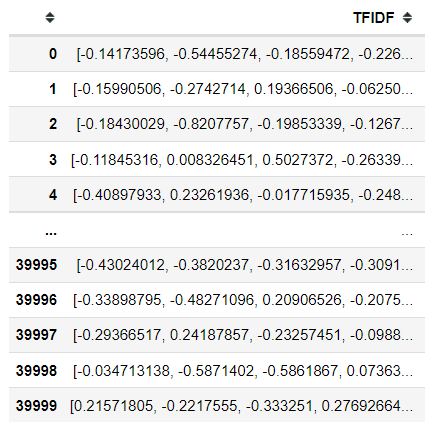
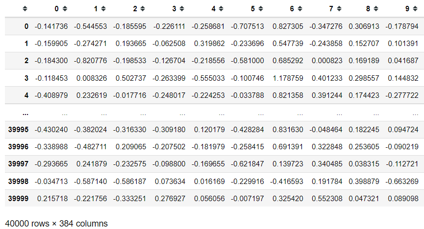
Figure 1 shows the raw features of the dataset. In this dataset, there are 40000 vectors and each vector is 384-dimensional. Figure 2 shows the features of the dataset after splitting. The processed dataset contains 40000 instances. Each instance has 384 factors to calculate, which is much easier than before.

3.2. The distribution of labels in datasets

Python programs are used to display the distribution of “positive” and “negative” in the train dataset and development dataset. The distribution is shown below (Figure 3).

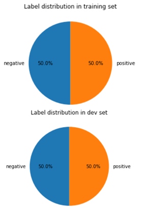
As is shown above, the distributions of the two labels are 50% respectively, which means the distribution is balanced and there is no bias.

4. Method and metrics

In this section, the baseline and machine learning paradigms are introduced.

4.1. Baseline

To assess models, a baseline is essential. The baseline in this study is based on 0-R, commonly known as the baseline for the majority class [9].

Since both labels have the same proportion, each of these labels can be the majority class. As a consequence, it makes a “positive” prediction for the first half and a “negative” prediction for another part, with the accuracy of this prediction serving as the baseline. This prediction takes absolutely no characteristic into account, making it appropriate as a baseline.

4.2. K-nearest neighbors

It is suited for K-Nearest Neighbors (KNN) on this preprocessed data. It firstly calculates each distance between every testing instance and every training instance, after which it chooses the K distances with the shortest values. The instance is then put into the K instances’ primary class [10].

The KNN does not require any extra presumptions or variables. Additionally, it is straightforward and typical for classification and simple to compare with other models.

4.3. Gaussian naive bayes

The prior and likelihood should be computed by using formulae in the Gaussian Naive Bayes (GNB) model. The forecast outcome of the testing case is the class with the highest probability following computations.

The GNB is appropriate because the attributes of the experiment are entirely numerical. It also has a mathematical theory foundation. It is an easy, quick, and precise method to evaluate the model.

4.4. Logistic regression

When using Logistic Regression (LR), which restricts the prediction range to [0,1], the sigmoid function, equation (1), is crucial. Additionally, in this study, the decision threshold is equal to 0.5. Boundary, which is dependent on computation, may forecast every class.

\( \frac{∂σ(z)}{∂z}=σ(z)[1-σ(z)] \) (1)

For binary classification, LR is acceptable. Because it involves less computing and is based on a probabilistic explanation and mathematical theory. Additionally, it makes predictions quickly and precisely. As a result, LR may be utilized for testing and training.

4.5. Evaluation metrics

The accuracy and the F1 are suitable for this experiment to evaluate the models.

4.5.1. Accuracy. As a measure of the percentage of accurate forecasts, accuracy is utilized. It contrasts expected and observed outcomes, counts the proportion of accurate outcomes, and computes the percentage. The most logical measure of a trained model's predictive power is accuracy, and it works well with balanced datasets.

4.5.2. F1. The model would be better if Precision and Recall are higher. They are in opposition to one another, though. In order to fully examine Precision and Recall, the F-score is used, as shown in equation (1). Precision and Recall would be treated equally when β = 1, as shown in equation (2).

\( {F_{β}}=\frac{(1+{β^{2}})PR}{{β^{2}}P+R} \) (2)

\( {F_{1}}=\frac{2PR}{P+R} \) (3)

The F1 tries to evaluate models different in accuracy and takes into account all of the model’s benefits and drawbacks.

4.6. Design of experiments

The benchmark for all models in this experiment is the specifically created baseline. Supervised learning with labeled datasets is carried out using KNN, GNB, and LR models. The accuracy and F1 of the development prediction are then produced [11].

Using semi-supervised learning and self-training, this experiment examines whether unlabeled data enhances the categorization of Twitter sentiment. The unlabeled dataset and the labeled dataset are mixed by self-training, and LR is chosen as the base estimator. The data that fall below the threshold criteria are then picked out and eliminated. Three models will be trained using this new dataset, and their accuracies and F1 scores will then be compared.

Comparing all of the computation results from the output above is important to arrive at an accurate and impartial conclusion. Controlling variables are used to assess different results reached in various circumstances.

5. Result

Different results of each situation are displayed in this section, and they are described as well.

5.1. Supervised learning

5.1.1. Positioning Figures and Tables. Figures and tables should be placed at the top and bottom of columns instead of the middle of columns. Large figures and tables may span across both columns. Figure captions should be below the figures; table heads should appear above the tables. Insert figures and tables after they are cited in the text. Use the abbreviation “Fig. 1”, even at the beginning of a sentence.

As shown in Table 1, both the accuracy and F1 of the baseline equal 0.506. Additionally, every performance exceeds the baseline. Because the features in the training dataset are not independent, LR has the best accuracy and F1, and GNB has the lowest, while KNN is represented by various K.

5.1.2. Semi-supervised learning. In Table 2, the LR has the best performance with semi-supervised learning. In Table 3, accuracy and F1 arrive at the highest value when the threshold equals 0.85 instead of 0.90, which means a higher threshold does not bring higher accuracy or F1. Besides, Table 4 tells the GNB has better performance when the threshold equals 0.80.

6. Discussion

6.1. Unlabeled data

In the real world, getting data is simple, but categorizing and labeling are expensive. As a result, there is far more unlabeled data than labeled data.

Unlabeled data must be included in the training set in order to make the most of the available data. It uses a different machine learning paradigm. For this experiment, semi-supervised learning is appropriate.

6.2. Semi-supervised learning

A small labeled dataset plus a sizable unlabeled dataset is used in semi-supervised learning to train models. 100000 unlabeled data points are not used. Labeled and unlabeled data can be used for self-training in semi-supervised learning to increase the training set [12].

Unlabeled data will produce findings with "confidence" after prediction. It will be included in a new training set with a labeled dataset if its "confidence" values above a threshold that the author specifies [13]. In this study, the threshold is trained using a default value of 0.8.

6.3. Evaluation

As shown in Tables 5, 6, and 7, KNN and LR perform better than GNB in supervised learning and semi-supervised learning.

6.4. Analysis

Accuracy and F1 increase insignificantly or drop. As shown in Tables 2, 3, and 4, it indicates that after semi-supervised learning, model accuracy and F1 have increased, supporting hypotheses. As the training set is increased, models get improved. The prediction of the dataset will theoretically become more accurate. But there are several exceptions in semi-supervised learning.

The data of metrics increases in these models are negligible. It is interesting to note that the semi-supervised GNB outcome drops when the threshold equals 0.6 (Table 6). The training dataset is larger than the initially labeled dataset by more than double. So, according to the development dataset, performance ought to greatly improve. However, as seen in the aforementioned data, the accuracy and F1 have reduced or just marginally risen, which is unexpected and calls further attention to what took place throughout the training.

6.4.1. Error propagation. Mistakes in prediction are unavoidable for every model. Even though the threshold is set during self-training, it is hard to completely eliminate prediction mistakes because this is a common occurrence. The new training set will contain incorrect pseudo-labels [14], and this incorrect data will influence models during training, decreasing prediction.

In other words, incorrect semi-supervised learning predictions will result in incorrect data in the next training set, which leads to inaccurate model output. Finally, the accuracy of forecasts will either somewhat improve or significantly deteriorate.

Since the proper labels of the sounds produced by incorrect predictions are unknown, they are challenging to identify and eliminate. However, there is still a solution to the spreading error issue:

With the new dataset, segmentation may be done with tougher thresholds [15]. The threshold of self-training can be split into several groups for independent training. As a result, the amount of introduced data steadily diminishes. Training and testing are then carried out independently. Setting the criterion to 0.85 in Table 3 results in the highest performance, which slightly declines at 0.9. They still outperform the outcomes of supervised learning. Due to the low amount of data provided to the training set by a high threshold, the training impact will be reduced but overall accuracy will rise.

6.4.2. Overfitting. Overfitting is a significant contributor to training-related mistakes. The experiment explicitly assessed the semi-supervised learning model's performance in predicting the training set and testing set in the same situation to see whether it was overfitting.

Table 8 shows that after training, the model is overfit. The model’s prediction of the development dataset is substantially less accurate since it resembled the training set too closely. Although training sets contain a lot of characteristics, not all of them are directly relevant to classification.

The most popular technique for minimizing the impact of overfitting is feature selection. It may be discovered that some traits are relevant to categorization by the computation of mutual information. Following the decision, it is possible to employ just features with a strong correlation, which can drastically reduce the number of features and the impact of overfitting.

7. Conclusion

This paper conducts comparative experiments on supervised learning, unsupervised learning, and semi-supervised learning. The experimental results show that, after introducing the unlabeled dataset, the accuracy and F1 of machine learning can be effectively improved. Moreover, semi-supervised learning can have both the high accuracy of supervised learning and the characteristics of using the unlabeled dataset. These two characteristics make it obtain a better training effect in the process of machine learning.

These unlabeled datasets are used in the form of pseudo-labels, and these pseudo-labels may cause error transmission and reduce the accuracy of the model. This is a cause of error propagation that cannot be ignored and has a greater impact on the effect of the model. Therefore, in the process of generating pseudo-labels, a method is needed to improve the accuracy of pseudo-labels, which still needs a period of time to explore in future studies.

References

[1]. Zhang, S., Li, X., Zong, M., Zhu, X. and Wang, R. Efficient kNN classification with different numbers of nearest neighbors. IEEE transactions on neural networks and learning systems 29(5), 1774–1785 (2017).
[2]. Ontivero-Ortega, M., Lage-Castellanos, A., Valente, G., Goebel, R. and Valdes-Sosa, M. Fast Gaussian Naïve Bayes for searchlight classification analysis. Neuroimage 163, 471–479 (2017).
[3]. Komarek, P. Logistic regression for data mining and high-dimensional classification. Carnegie Mellon University (2004).
[4]. Eisenstein, J., O’Connor, B., Smith, N. A. and Xing, E. P. A latent variable model for geographic lexical variation. In Proceedings of the 2010 Conference on Empirical Methods in Natural Language Processing (EMNLP 2010), Cambridge, USA, 1277–1287 (2010).
[5]. Blodgett, S. L., Green, L., and O’Connor, B. Demographic dialectal variation in social media: A case study of African-American English. In Proceedings of the 2016 Conference on Empirical Methods in Natural Language Processing, Austin, Texas, Association for Computational Linguistics, 1119–1130 (2016).
[6]. Deri, A. and Knight, K. How to make a frenemy: Multitape FSTs for portmanteau generation. In Human Language Technologies: The2015 Annual Conference of the North American Conference of the North American Chapter of the ACL, Denver, USA, 206–210 (2015).
[7]. Das, K. and Neuramanteau, S. A neural network ensemble model for lexical blends. In Proceedings of The 8th International Joint Conference on Natural Language Processing, Taipei, Table 8. Test for overfitting. Semi-supervised, K=40 Accuracy F1 Prediction of development set 0.69125 0.69083 Prediction of training set 0.85259 0.85248 Taiwan, 576–583 (2017).
[8]. Cook, P. and Stevenson, S. Automatically identifying the source words of lexical blends in English. Computational Linguistics 36(1), 129–149 (2010).
[9]. Choudhary, R. and Gianey, H. K. Comprehensive review on supervised machine learning algorithms. In 2017 International Conference on Machine Learning and Data Science (MLDS), IEEE, 37-43 (2017).
[10]. Guo, G., Wang, H., Bell, D., Bi, Y. and Greer, K. KNN model-based approach in classification. In OTM Confederated International Conferences. On the Move to Meaningful Internet Systems. Springer, Berlin, Heidelberg, 986-996 (2003).
[11]. Singh, A., Thakur, N. and Sharma, A. A review of supervised machine learning algorithms. In 2016 3rd International Conference on Computing for Sustainable Global Development (INDIACom), IEEE, 1310-1315 (2016).
[12]. Van Engelen, J. E. and Hoos, H. H. A survey on semi-supervised learning. Machine Learning 109(2), 373-440 (2020).
[13]. Rosenberg, C., Hebert, M. and Schneiderman, H. Semi-supervised self-training of object detection models (2005).
[14]. Lee, D. H. Pseudo-label: The simple and efficient semi-supervised learning method for deep neural networks. In Workshop on challenges in representation learning, ICML 3(2), 896 (2013).
[15]. De Sousa Ribeiro, F., Calivá, F., Swainson, M., Gudmundsson, K., Leontidis, G. and Kollias, S. Deep bayesian self-training. Neural Computing and Applications 32(9), 4275-4291 (2020).
Cite this article
Ren,Y. (2023). Sentiment Prediction by a Classifier. Applied and Computational Engineering,8,18-25.
Data availability
The datasets used and/or analyzed during the current study will be available from the authors upon reasonable request.
Disclaimer/Publisher's Note
The statements, opinions and data contained in all publications are solely those of the individual author(s) and contributor(s) and not of EWA Publishing and/or the editor(s). EWA Publishing and/or the editor(s) disclaim responsibility for any injury to people or property resulting from any ideas, methods, instructions or products referred to in the content.
About volume
Volume title: Proceedings of the 2023 International Conference on Software Engineering and Machine Learning
© 2024 by the author(s). Licensee EWA Publishing, Oxford, UK. This article is an open access article distributed under the terms and
conditions of the Creative Commons Attribution (CC BY) license. Authors who
publish this series agree to the following terms:
1. Authors retain copyright and grant the series right of first publication with the work simultaneously licensed under a Creative Commons
Attribution License that allows others to share the work with an acknowledgment of the work's authorship and initial publication in this
series.
2. Authors are able to enter into separate, additional contractual arrangements for the non-exclusive distribution of the series's published
version of the work (e.g., post it to an institutional repository or publish it in a book), with an acknowledgment of its initial
publication in this series.
3. Authors are permitted and encouraged to post their work online (e.g., in institutional repositories or on their website) prior to and
during the submission process, as it can lead to productive exchanges, as well as earlier and greater citation of published work (See
Open access policy for details).