1. Introduction

Autism spectrum disorder (ASD) is a neurodevelopmental disorder difficult to diagnose. The current psychiatric diagnostic process is based simply on observing the behavioral symptoms [1] neither with enough knowledge of the neurological mechanisms behind autism spectrum disorder, nor suitable for quantitative diagnosis and may lead to false diagnosis [2].

In recent decades, advances in neuroimaging technologies have made it easy to measure those pathological changes related to the brain with autism spectrum disorder. The fMRI data has the features that tell the difference between ASD brain and healthy controls. Resting state fMRI reflects the functional relationship between areas of the brain. The fluctuations in blood oxygenation or flow indicate the correlation of low-frequent undulation on resting state fMRI. It illustrates functional connectivity of the brain [3]. An average correlation of the time series between the regions of interest is calculated in order to investigate the link between different areas of the brain. The correlation is used to form a connectivity matrix. Nevertheless, the differences between the brain with ASD and the healthy controls are too subtle to help detect biomarkers applying traditional computational or statistical methods. Progressive machine-learning solutions provide a systematic method to develop self-acting solutions for classifying objective and study the delicate patterns demonstrated by the data that may be particular to the brains with ASD [4]. In the case of mental disease states, researchers have identified patients with brain activation associated with schizophrenia [5], with autism [6], and with depression [7].

FIGURE 1 demonstrates the areas of Gray Matter and White Matter using the T1-weighted MRI brain-imaging scan to map the structural changes of brain development. The White Matter functions as the creation of new connections for the highly dynamic growth process. The Gray Matter, containing numerous cell bodies and few myelinated axons, is distinguished from the White Matter. The job of the Gray Matter is to eliminate or prune the unused brain cells. Below this 11-year-old boy’s brain imaging with autism clearly shows that there is a delay in the growth rate of the White Matter, which is also responsible for the connecting brain regions for social and language abilities. At the same time, the unused cell from the Gray Matter is not sufficiently pruned away, leaving trouble in the putamen for learning and the anterior cingulate for regulating emotions and cognitions.

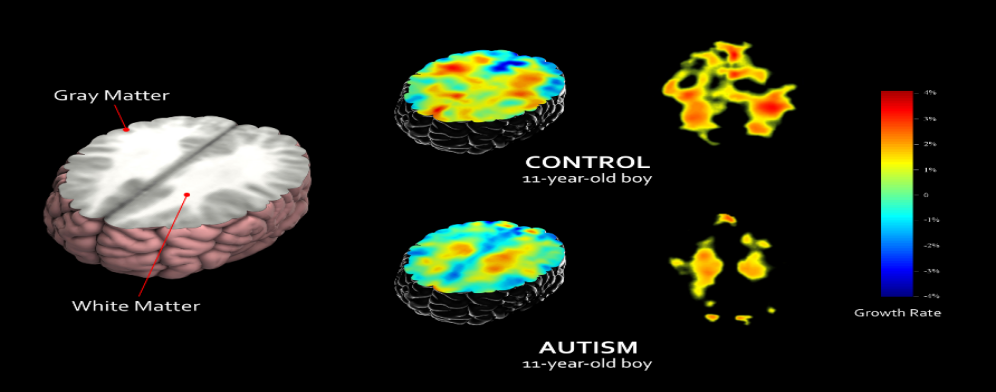
Figure 1. Control and autism subject comparison (UCLA Laboratory of Neuro Imaging).

Studies have identified individuals as autistic or healthy from their resting state fMRI brain activation with almost 97% accuracy single sites applying machine-learning algorithms to ASD brain imaging data. They also discovered a psychological driven brain activation pattern. The pattern was found in control participants and nearly undiscovered in autistic patients [6]. A proviso of studies applying supervised machine learning to brain imaging is their relatively small data size. Classification accuracy plummets in larger databases and if the source of the data is different [8]. A majority of studies have utilized supervised learning methods to integrate brain imaging with machine learning. When selecting the features during the process of supervised learning, much subjectivity is added to the experiment, which may be a hindrance to the comparison of the results from different studies. The choice of the labels and of the features of the training set are decided by not only a priori hypothesis but also exploratory trials; therefore, they are based on subjectivity to certain extent [9]. If we extract features more objectively, we might have a refreshed insight into the function of brain that depends less on experimenters and rests more with data. According to the previous studies, deep learning is promising for brain imaging applications in the clinical field [10].

To achieve more quantitative diagnosis in this field, an advanced and scalable deep-learning architecture, which helps discover reliable biomarkers of mental health disorders is needed. This project explored a deep-learning architecture that integrated supervised machine-learning methods with unsupervised ones for differentiating autistic patients from health controls with the resting state fMRI data. The second goal of this project was to research the neural patterns regarding autism spectrum disorder that is most substantial to the classification and thus help improve our perception of the neurobiological biomarkers of the autistic brain. Furthermore, these methods proposed in the project can help to detect ASD more accurately and earlier.

The structure of the paper is: In section 2, we discussed some previous relevant studies and several relevant state-of-the-art tools. In section 3, we proposed all the feature extraction methods, data-augmentation methods, and deep learning methods we have tried. In section 4, we compare the performance of our new methods with the methods proposed in the previous related papers. In section 5, we conclude our experiments and discuss the future work.

2. Related work

Previous studies have demonstrated some models to classify Autism in their research. Heinsfeld et al. [9] proposed a model obtaining 70% accuracy for classifying 1,035 subjects but obtaining only 52% accuracy for classifying each of the 17 sites contained in the ABIDE dataset. Eslami et al. [4] suggested an architecture model called ‘ASD-DiagNet’ based on that proposed by Heindfeld et al. [9]. In ASD-DiagNet, the auto-encoder and the single layer perceptron are trained in a joint method for performing feature selection and the later classification. Almuqhim et al. [11] proposed a model called ‘ASD-SAENet’ based on ‘ASD-DiagNet’. ASD-SAENet is comprised of a sparse auto-encoder and a deep neural network. The highest accuracy of the models mentioned above is around 70%. Generally, the inspiration of our model came from the study of ‘ASD-SAENet’ [11].

Many other methods were tried aside from those proposed in the previous papers. Basically, an attempt at modifying the ‘ASD-DiagNet’ was made to advance the classifying operation. In the process of data augmentation, the ‘ASD-DiagNet’ used a basic linear interpolation method called Synthetic Minority Over-sampling Technique (SMOTE). This data augmentation method doubled the size of the training set. What was modified here is to replace SMOTE with the Mixup method -- A linear augmentation method proposed by MIT. In the process of feature selection, an autoencoder was used to extract a lower dimensional feature representation. A Sparse Autoencoder or a Variational Autoencoder was chosen instead of a general Autoencoder to alleviate the influence of overfitting in the results. The Variational Autoencoder could help with introducing reconstructed input to the dataset. Concerning the classification assignment, the ‘ASD-DiagNet’ implemented a single-layer perceptron (SLP) that used the autoencoder's bottleneck layer as input. Instead, we replace the single layer perceptron with a deep neural network as the classifier.

3. Material & method

3.1. Dataset

As MRI imaging is commonly used for brain disorders, the fMRI is the method to evaluate cognitive activity by monitoring the blood flow to specific sections of the brain. Where the blood flow increases, the neurons will be active. In fMRI data, different brain volumes are represented by a series of little cubic elements named voxels. Every voxel’s activity is tracked over time to extract the time series as an eigenvector. In this study, brain disorder is analyzed using a fMRI technology called rs-fMRI (resting state fMRI), which is widely applied in brain diseases evaluation. Those rs-fMRI data are preprocessed by a pipeline provided by ABIDE initiative and used for training and testing, this dataset consists of 1035 samples including 505 subjects with Autistic patients and 530 normal individuals.

The dataset applied in our study is preprocessed by a pipeline called C-PAC (Configurable Pipeline for the Analysis of Connectomes) which parcellated the brain into 200 functionally homogeneous regions using spatially constrained spectral clustering algorithm (CC-200) [12]. Generally speaking, most research on ASD diagnosis using machine learning technology only consider a subset of the dataset. Or the research may include other demographic information other than fMRI data in the model. However, a linear augmentation method was applied in this study to expand the dataset using the available original sets which consists of samples collected from 17 different sites. During the evaluation phase, we firstly trained and tested the model with whole 1,035 samples. Then, the model was evaluated using the samples from each site separately [4]. Furthermore, in order to prove the robustness of the model and its ability to adapt to different data sets, we also collected time series extracted from five sets of ROIs (Region of interest) based on five varied atlases preprocessed by other pipelines to evaluate the performance of the model.

3.2. Feature extraction

The connectivity among different brain regions is often used in fMRI assessment and is proved to be an important feature of fMRI pattern recognition. In our study, correlation was taken as an index to measure the connectivity of different brain regions.

Pearson’s correlation is widely applied for measuring the functional connectivity in fMRI data among all correlation methods [13-15]. It represents the linear relationship among time series of different regions. The other correlation measure is the Spearman correlation coefficient. It assesses the monotonic relationship between two variables which can better reflect the dependence of different regions of the brain. So, we use Spearman correlation to approximate the functional connectivity in fMRI data. Given the two series, \( R \) and \( S \) , each of length \( T \) , the Spearman’s correlation could be generated using the equation below:

\( {ρ_{s}}=\frac{\sum _{i=1}^{N}({R_{i}}-\bar{R})({S_{i}}-\bar{S})}{{[\sum _{i=1}^{N}{({R_{i}}-\bar{R})^{2}}\sum _{i=1}^{N}{({S_{i}}-\bar{S})^{2}}]^{\frac{1}{2}}}}=1-\frac{6\sum d_{i}^{2}}{N({N^{2}}-1)} \)

where \( \bar{R} \) , and \( \bar{S} \) are the means of the series \( {R_{i}} \) and \( {S_{i}} \) respectively, \( {d_{i}}={R_{i}}-{S_{i}} \) . FIGURE 2 illustrates the process of the feature extraction. We calculate all pairwise correlations to generate a matrix \( {C_{n×n}} \) . As for the atlas we use is CC200 which divides the brain into 200 regions (n=200), and it finally generates a 200 × 200 matrix. Since the matrix we calculated is diagonal symmetric, we decide to use the matrix’s upper triangle only and transform it into a one-dimensional vector as the features of Autoencoder. All those pairs finally result in the vectors with \( \frac{n(n-1)}{2}=19,900 \) values. In order to lower the dimension of the eigenvector, we applied the same method as Eslami et al. [16], and only selected the \( \frac{1}{4} \) maximum and \( \frac{1}{4} \) minimum of the average correlation array as mask to obtain the eigenvector with 9950 values as the input of each subject.

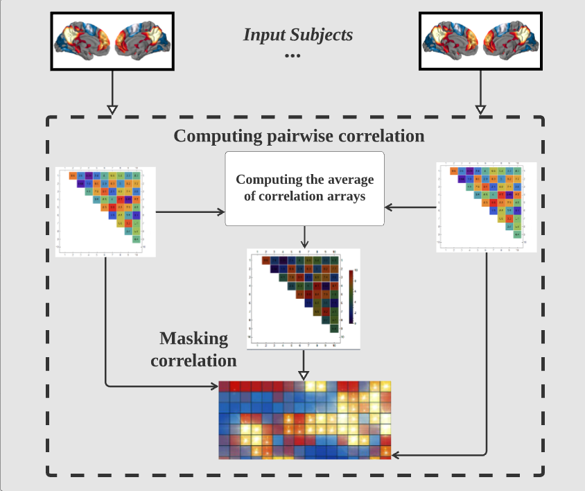
Figure 2. Workflow of feature extraction.

3.3. Model architecture

The diagram FIGURE 3 illustrates the overall model architecture that the paper has mainly focused on. From step A. Data Augmentation to step B using autoencoder with Deep Neural Network including B.1 Sparse Autoencoder with Deep Neural Network and B.2 Variational Autoencoder with Deep Neural Network. Later moving on to step C. Cross Validation through K-folding. More detailed construction of each step is discussed in the following sections.

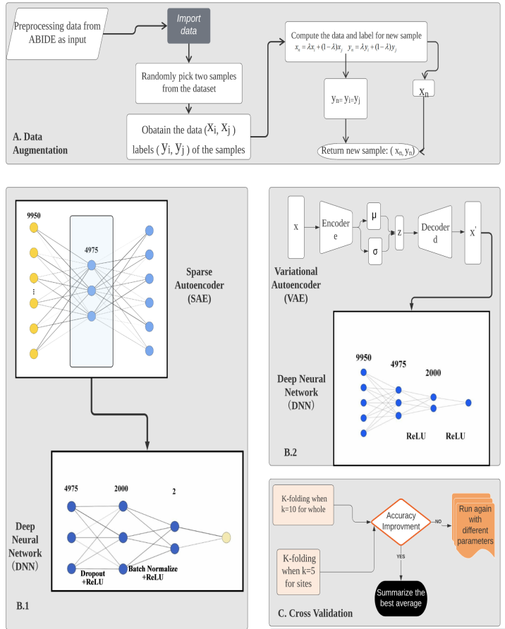
Figure 3. Model architecture.

3.4. Data augmentation

To reduce the impact of insufficient training set on the generalization ability of the model, this work uses a linear data augmentation method called ‘Mixup’ to expand our dataset.

Mixup is a linear augmentation method based on the principle of Vicinal Risk Minimization (VRM), which uses linear interpolation to generate new sample data. In VRM, human knowledge is needed to describe the neighborhood or vicinity around each sample in the training set. Then, additional virtual samples can be extracted from the vicinity distribution of training samples to expand the support of training distribution. For example, when performing classification of the image data, the vicinity of an image is usually defined as a set of its horizontal reflection, mild rotation, and slight scaling. Data augmentation is therefore considerably resulting in the improvement of generalization.

The research in Zhang et al. [17] proposed a Mixup distribution:

\( μ(\widetilde{x},\widetilde{y}|{x_{i}},{y_{i}})=\frac{1}{n}\sum _{j}^{n}E[δ(\widetilde{x}=λ∙{x_{i}}+(1-λ)∙{x_{j}},\widetilde{y}=λ∙{y_{i}}+(1-λ)∙{y_{j}})] \)

where \( λ~Beta(α,α) \) , for \( α∈(0,∞) \) . To be concrete, the virtual feature-target vector is generated by sampling from the mixed vicinal distribution:

\( {x_{n}}=λ{x_{i}}+(1-λ){x_{j}} \)

\( {y_{n}}=λ{y_{i}}+(1-λ){y_{j}} \)

Where ( \( {x_{n}} \) , \( {y_{n}} \) ) is the new virtual data generated by linear interpolation, ( \( {x_{i}} \) , \( {y_{i}} \) ) and ( \( {x_{j}} \) , \( {y_{j}} \) ) are the two samples randomly selected in the training set. \( {x_{n}} \) is the random generation of new data samples, and \( {y_{n}} \) is the label of \( {x_{n}} \) . It should be noted that the range of \( {y_{n}} \) generated by mixup is [0,1], but the labels of our samples are ‘0’ and ‘1’ (‘0’ means healthy people and ‘1’ means ASD-patients). Therefore, this method set the value of the label to be the same as that of its nearest neighbor label, so the new sample label obtained is ‘0’ or ‘1’.

The FIGURE 4 flowchart shows how we generated new samples by Mixup:

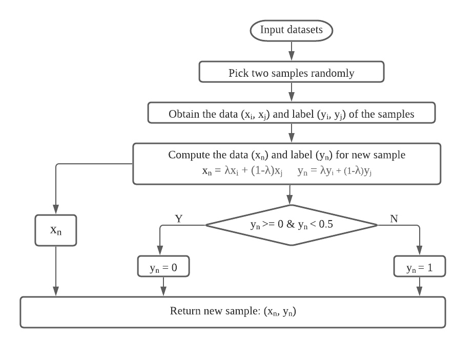
Figure 4. Generate new samples by Mixup.

In addition to interpolating between two random samples, we also tried to interpolate between the nearest neighbors. We took similarity as a measure of the distance between two samples to obtain the nearest neighbor. In order to calculate the similarity among samples, we applied a technology called Extended Frobenius Norm (EROS) which has proved to be an effective way to measure the similarity of fMRI data in previous studies. We use this method to find the k-nearest neighbors of our training samples to obtain higher classification accuracy.

As FIGURE 5 shows below, after selecting each sample’s nearest neighbors in the training set, we randomly picked one among them, the new sample and label is generated using Mixup between the chosen neighbor and original sample. The reason why we chose k=5 is that no better results have been observed by changing the value of k in our experiment. The label of the new sample is consistent with the original sample and its neighbors.

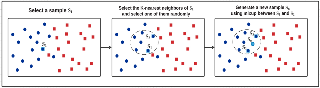
Figure 5. Interpolation between nearest neighbors.

Experiments show that interpolation between neighbors can reach higher classification accuracy than between two random samples. So, we choose the former as our final data augmentation method. All results of the testing phase are achieved by this method.

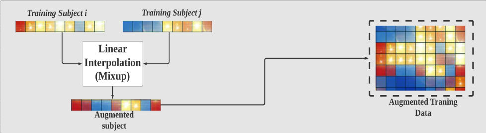
Figure 6. Generate new feature vectors of training samples.

As FIGURE 6 shows, subject i and subject j are the feature vectors of the random sample and its random neighbor. In this work, these two feature vectors were used to generate the new vectors of training samples by linear interpolation method. Since each sample in the dataset will be used to generate a new sample, the size of our training dataset will be doubled after data augmentation. In fact, we have tried to generate multiple new samples with the same original samples, but we did not obtain a significant change of the result.

While learning from the labels of corruption or facing hostile examples, Mixup can enhance the robustness of neural networks even though its principle is very simple. In the meanwhile, this method improves the generalization ability of speech and tabular data and can be used to stabilize the training of Deep Neural Networks and other networks.

3.4.1. Sparse autoencoder and deep neural network. Generally, autoencoders are key to the development of deep learning as it is part of the unsupervised learning model. The Sparse Autoencoder is one of the autoencoders whose training specification includes a sparsity penalty. In this combined algorithm with Deep Neural Networks, the loss function is constructed through penalizing activation of hidden layers for a few active nodes while the sample is fed into the network. The autoencoder is learning the latent representation rather than the redundant from the input dataset. Instead of using the common \( {L_{1}} \) loss function, the loss function that is implemented in the proposed method is through the Huber loss function using delta data. The Huber loss is also known as Smooth \( {L_{1}} \) loss for its transition point option equals one. The formula is as below:

\( E=\frac{1}{N}\sum _{i=1}^{N}\sum _{j=1}^{k}{smooth_{L1}}({\hat{y}_{ij}}-{y_{ij}}) \)

The benefit of using the sparse autoencoder is that the model can acquire finer representations and activations are sparser, preventing the data from overfitting. With the \( {L_{1}} \) regulation, the sparse autoencoder is better performing than other general autoencoders. The encoding process generates lower dimensional data which contains useful patterns from the original input data. Thus, the new features for classification can fully operate within the smaller data sizes. The input of the deep neural network arises from the bottleneck of the Sparse Autoencoder.

The deep neural network will be composed of two hidden layers where the sizes are 2,000 and 2 units respectively. To avoid overfitting of the model, the method of Dropout was used between the first and the second fully connected layers. To accelerate the training speed and minimize the error brought about by the careless initialization of the parameters [18], a batch normalization layer was added between the second and the third fully connected layers to remove the ill effects of the internal covariate shift. A rectified linear unit (ReLU) was also applied to activate the units after each layer. The ReLU can expand the sparsity of the network so that the extracted features will be more representative. Consequently, the network will have improved generalization ability. Furthermore, ReLU can solve the missing-gradient problem present in the back-propagation process of the deep neural network. The loss of the deep neural network is calculated with Binary Cross Entropy. The equation of the Binary Cross Entropy is shown below:

\( {H_{p}}(q)=-\frac{1}{N}\sum _{i=1}^{N}{y_{i}}∙log(p({y_{i}}))+(1-{y_{i}})∙log(1-p({y_{i}})) \)

The Sparse Autoencoder and the deep neural network developed characteristic extraction while optimizing the determination of classifiers after training concurrently.

3.4.2. Variational autoencoder and deep neural network. Variational autoencoders (VAE) are variational Bayesian procedures with a diverse distribution as prior, and a posterior approximated by an artificial neural network, constructing the variational encoder-decoder model. The Variational Autoencoder differs from the common autoencoder as the VAE introduces mapped input to distribution and the bottleneck vector is replaced by two various vectors including the standard deviation of the distribution and the mean of the distribution. The main objective of the VAE is the Kullback-Leibler Divergence also known as KL divergence, calculated as below:

\( {D_{KL}}(q({x_{i}})||p({x_{i}}))=\int q({x_{i}})log\frac{q({x_{i}})}{q({x_{i}})}dz \)

The KL divergence is measuring the differences between two distributions. To minimize the generative modal parameters and reduce the reconstruction error within the network between input and output (reconstructed input). Equivalent to minimizing the negative log-likelihood commonly found in most optimizations, the objective is to minimize the distribution distances between the real and estimated posterior. Therefore, the loss function Evidence Lower Bound (ELBO) is written as:

\( {L_{ELBO}}(x;θ,Φ) ∶= -\underset{Likelihood}{\underbrace{\int log{p_{θ}}(x|z){q_{Φ}}(z|x)dz}}+\overset{Latent space distance}{\overbrace{{D_{KL}}({q_{Φ}}(z|x)||p(z))}} \)

In order to make the ELBO loss function reliable for training the data, the Stochastic sampling operation extracts from the latent space, which is a series of multivariate Gaussian Distributions, thus dedicating the probabilistic decoder as follows:

\( z~{q_{Φ}}(x)=N(μ,{σ^{2}}) \)

Based on the calculation of the variational autoencoder, the deep neural network takes the filtered data with random variables processed by VAE as reconstructed input to train further. The deep neural network with the two hidden layers where the units are 4,975 and 2,000 respectively. ReLU was used between the fully connected layers. It has been confirmed by Diederik et al., [19] that Adam shows better convergence than other methods in the process of stochastic regularization in multi-layer neural networks. Adam optimizer is thus applied to update the parameters built upon the computed gradients.

3.5. Model validation

To test our model for its performance, we have adapted the model validation method that the previous work has used which is the K-folding cross validation. The validation set is extracted from training set data but does not train it. The original data is divided into K folds, k=10. Each of the k sets is to evaluate the final result and calculate the Mean Squared Error combined with the means. For each individual site, the validation method is used through K-folding when k=5 as other previous studies used the same values.

4. Experiment and results

TABLE 1 demonstrates the highest anticorrelation areas for ASD subjects, FIGURE 7 highlights these areas in the brain image for visualization. The ASD patients have characteristics of the brain function that are decreased anterior-posterior connectivity and the posterior regions are increased corresponding to the connectivity switches in the brain. Due to the one-dimensional aspect of the ABIDE dataset and the lack of sponsored clinical facility, the visualization of the fMRI result is adapted from the previous studies. These studies are the foundation for a data-driven theory that is heavily based on the brain-imaging underconnectivity in ASD research which has also been associated with indices of corpus callosum and morphometric brain structures [20]. The frontal-temporal sections like the middle temporal and inferior frontal; the fusiform gyrus region and the orbital cortex region, posterior such as the supramarginal gyrus area, and anterior with the paracingulate gyrus region of the ASD subjective brains have anticorrelation that reflects underconnectivity. The characteristics of the underconnectivity is the basis of the proposed model which contributes to the classification procedures.

Table 1. Summary of the highest anticorrelation areas for ASD subjects.

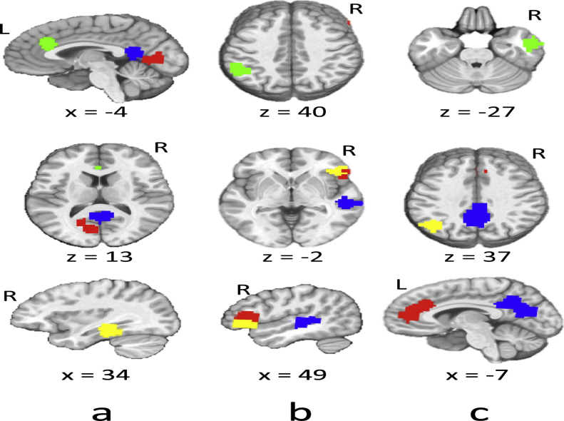
Figure 7. Related Summary of the highest anticorrelation areas brain imaging.

4.1. Running time

Based on the previous studies, the running time by ASD-DiagNet is around 41 minutes, around 7h and 48 minutes by the Support Vector Machine learning (SVM), around 17 min with random forest approach, and 6 hours by the method of Heinsfeld et al. [9]. The proposed method of B.1 runs 2 hours and 38 minutes while the other method B.2 runs 3 hours and 19 minutes. ASD-DiagNet in general performs faster in speed of training and validation, but our proposed methods are relatively fast compared to the SVM and Heinsfeld et al. [9].

4.2. General accuracy

In the proposed experiment of our method, there are two different approaches with both method B.1 and B.2. The ABIDE dataset, including 1035 subjects, has patients from various sites. Therefore, the result is summarized from both individual sites and the generalization across different data acquisition sites. Different performance compared to the past models through the three significant values Accuracy, Sensitivity and Specificity. The three values measure different aspects of the dataset. To be more specific, the value of Accuracy determines the percentage of correctly classified subjects, whether or not the actual ASD is classified as ASD, and the control group is classified as healthy. The second value of Sensitivity measures the percentage of real ASD patients which are accurately considered carrying the ASD. The last value of Specificity illustrates the percentage of successfully classified healthy subjects.

As TABLE 2 indicates, the two proposed methods in this work all have much better results than the methods from previous studies by Heinsfeld et al., [9] and Eslami et al., [4]. Since the limitation of the dataset, the final result is extracted from the best performances from each cross validation that the trained data could generate, and then calculate the average from the extracted results. FIGURE 8 compares the ASD classification accuracy of the proposed methods and the previous methods. The B.1 method has better accuracy and sensitivity value in contrast to the result from the B.2 method. The specificity from both methods is equal.

Table 2. The comparison between the current method with the previous work’s method like ASD-SAENet and ASD-DiagNet.

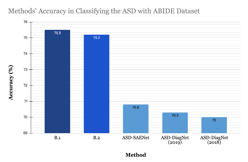
Figure 8. Method’s Accuracy in Classifying the ASD with ABIDE Dataset.

4.3. Individual site’s accuracy

After testing the accuracy result, the accuracy for each individual medical/university site that is within the data is also important. TABLE 3 shows the comparison between the results of method B.1 and method B.2. Method B.1 is the method that uses Sparse Autoencoder with Mixup data augmentation and deep neural network. Method B.2 is the method of using Variational Autoencoder instead of autoencoder enlarging the original dataset with reconstructive input.

To evaluate further, the medical/university acquisition sites for individual accuracy are calculated between the proposed methods B.1 and B.2. Through comparison between the classification accuracy of the two methods among 17 sites, we found out that B.2 using Variational Autoencoder is a little bit better than B.1 using Sparse Autoencoder on the average scale. Out of 17 acquisition sites, there are equal numbers of sites for both B.1 and B.2 methods to shine, eight sites that work better with SAE, the other eight sites work better with VAE. There is one site that works equally between SAE and VAE. However, the B.2 method has significant accuracy when training the OHSU sites. For the OHSU site, it is the sample collected from Oregon Health and Science University. The sample size has a total number of 28 people ranging from eight to fifteen years old. The control group is around 15 people, whereas the Autism patients are 13 people. This site includes data that is suitable to the model of VAE. After the reconstructed input, the accuracy is higher. Several sites which have lower accuracy despite the difference in method are MaxMun, Trinity which indicate that these two datasets have more variability that are absent in other sites. The MaxMun is the data from the Ludwig Maximilians University Munich while Trinity is the Trinity Centre for Health Sciences. Both sites have more people in the control group than the targeted autism group; the imbalance between the two might cause the accuracy to be lower as well.

Table 3. The accuracy through the current model B.1 (SAE+MIXUP+DNN) and model B.2 (VAE+MIXUP+DNN) for each imaging site of ABIDE dataset.

Table 3. (continued).

5. Conclusion

In this work, the data set from ABIDE consists of fMRI data provided by 17 different sites. Each dataset of the 17 sites was collected from patients with different scanning methods and devices. To avoid the overfitting of the results of the model, Mixup was applied to enlarge the dataset. In order to reduce the number of the features, Sparse Autoencoder is used before the process of classification. A deep neural network functioned as a classifier that got its inputs from the outputs of the encoding process of the Sparse Autoencoder. Between the linear fully connected layers in the deep neural network were confirmed methods like Dropout and Batch Normalization to further reduce the possibility of overfitting. In the second model, the deep neural network functioning as a classifier took the filtered data with random variables processed by VAE as reconstructed input to train further. Rectified Linear Units were added between the linear fully connected layers as activation functions. The accuracy of the results of the “Mixup+SAE+DNN” and “Mixup+VAE+DNN” are about 75.5% and 75.2% respectively, which outperformed the other state-of-the-art method by 4.7% and 4.4%. The further significance of this project is to help develop our perception of the neurobiological foundation of the ASD.

Multiple sites with different subjects, scanning procedures and equipment compared to single-site datasets [8] added noise to the brain-imaging dataset that disputes the classification performance. However, the achievement of a reliable classification accuracy without the noise shows prospects for the machine learning utilization in later clinical datasets. The future application of machine learning will help identify mental disorders of other kinds [9].

Data availability statement

The datasets analyzed for this study can be found in the ABIDE-I repository.

Acknowledgement

Wenhan Han, Wenzhu Shao and Yaluo Wang contributed equally to this work and should be considered co-first authors.

References

[1]. Nickel, R. E., & Huang-Storms, L. (2015, September 28). Early Identification of Young Children with Autism Spectrum Disorder. Indian Journal of Pediatrics. https://link.springer.com/article/10.1007/s12098-015-1894-0.
[2]. Baio, J., Wiggins, L., Christensen, D. L., Maenner, M. J., Daniels, J., Warren, Z., Kurzius-Spencer, M., Zahorodny, W., Robinson Rosenberg, C., White, T., Durkin, M. S., Imm, P., Nikolaou, L., Yeargin-Allsopp, M., Lee, L.-C., Harrington, R., Lopez, M., Fitzgerald, R. T., Hewitt, A., … Dowling, N. F. (2018, April 27). Prevalence of Autism Spectrum Disorder Among Children Aged 8 Years - Autism and Developmental Disabilities Monitoring Network, 11 Sites, United States, 2014. Morbidity and mortality weekly report. Surveillance summaries (Washington, D.C. : 2002). https://www.ncbi.nlm.nih.gov/pmc/articles/PMC5919599/.
[3]. Biswal, B., Yetkin, F.Z., Haughton, V.M., Hyde, J.S., (1995). Functional connectivity in the motor cortex of resting human brain using echo-planar MRI. Magn. Reason. Med. 34(4), 537-541.
[4]. Eslami, T., Mirjalili, V., Fong, A., Laird, A. R., & Saeed, F. (2019, January 1). ASD-DiagNet: A Hybrid Learning Approach for Detection of Autism Spectrum Disorder Using fMRI Data. Frontiers. https://www.frontiersin.org/articles/10.3389/fninf.2019.00070/full.
[5]. Yang, J., et al., (2010). Common SNPs explain a large proportion of the heritability for human height. Nat. Genet. 42(7), 565-569.
[6]. Just, M.A., Cherkassky, V.L., Buchweitz, A.,Keller, T.A., Mitchell, T.M., 2014. Identifying autism from neural representations of social interactions: neurocognitive markers of autism. PLoS ONE 9 (12), 1-22.
[7]. Craddock, R.C., Holtzheimer, P.E., Hu, X.P., Mayberg, H.S., (2009). Disease state prediction from resting state functional connectivity. Magn. Reason. Med. 62 (6), 1619-1628.
[8]. Nielsen, J. A., Zielinski, B. A., Fletcher, P. T., Alexander, A. L., Lange, N., Bigler, E. D., ... & Anderson, J. S. (2013). Multisite functional connectivity MRI classification of autism: ABIDE results. Frontiers in human neuroscience, 7, 599.
[9]. Heinsfeld, A. S., Franco, A. R., Craddock, R. C., Buchweitz, A., & Meneguzzi, F. (2018). Identification of autism spectrum disorder using deep learning and the ABIDE dataset. NeuroImage:
[10]. Plis, S.M., et al., (2014). Deep learning for neuroimaging: a validation study. Front. Neurosci. 8 (August), 229.
[11]. Almuqhim, F., & Saeed, F. (2021). ASD-SAENet: A Sparse Autoencoder, and Deep-Neural Network Model for Detecting Autism Spectrum Disorder (ASD) Using fMRI Data. Frontiers in computational neuroscience, 15, 654315. https://doi.org/10.3389/fncom.2021.654315
[12]. Zhan Y, Wei J, Liang J, Xu X, He R, Robbins TW, Wang Z. Diagnostic Classification for Human Autism and Obsessive-Compulsive Disorder Based on Machine Learning From a Primate Genetic Model. Am J Psychiatry. 2021 Jan 1;178(1):65-76. doi: 10.1176/appi.ajp.2020.19101091. Epub 2020 Jun 16. PMID: 32539526.
[13]. Liang X, Wang J, Yan C, Shu N, Xu K, Gong G, He Y. Effects of different correlation metrics and preprocessing factors on small-world brain functional networks: a resting-state functional MRI study. PLoS One. 2012;7(3):e32766. doi: 10.1371/journal.pone.0032766. Epub 2012 Mar 6. PMID: 22412922; PMCID: PMC3295769.
[14]. Baggio HC, Sala-Llonch R, Segura B, Marti MJ, Valldeoriola F, Compta Y, Tolosa E, Junqué C. Functional brain networks and cognitive deficits in Parkinson's disease. Hum Brain Mapp. 2014 Sep;35(9):4620-34. doi: 10.1002/hbm.22499. Epub 2014 Mar 17. PMID: 24639411; PMCID: PMC6869398.
[15]. Zhang, Y., Zhang, H., Chen, X., Lee, S. W., & Shen, D. (2017). Hybrid high-order functional connectivity networks using resting-state functional MRI for mild cognitive impairment diagnosis. Scientific reports, 7(1), 1-15.
[16]. Eslami, T., and Saeed, F. (2019). “Auto-ASD-network: a technique based on deep learning and support vector machines for diagnosing autism spectrum disorder using fMRI data,” in Proceedings of ACM Conference on Bioinformatics,Computational Biology, and Health Informatics (Niagara Falls, NY: ACM).
[17]. Zhang, H., Cisse, M., Dauphin, Y. N., & Lopez-Paz, D. (2017). mixup: Beyond empirical risk minimization. arXiv preprint arXiv:1710.09412.
[18]. Ioffe, S. & Szegedy, C.. (2015). Batch Normalization: Accelerating Deep Network Training by Reducing Internal Covariate Shift. Proceedings of the 32nd International Conference on Machine Learning, in Proceedings of Machine Learning Research 37:448-456 Available from http://proceedings.mlr.press/v37/ioffe15.html .
[19]. D.P. Kingma and J.L. Ba, Adam: A Method for Stochastic Optimization. San Diego: The International Conference on Learning Representations (ICLR), 2015.
[20]. Just, M. A., Cherkassky, V. L., Keller, T. A., Kana, R. K., & Minshew, N. J. (2007). Functional and anatomical cortical underconnectivity in autism: evidence from an FMRI study of an executive function task and corpus callosum morphometry. Cerebral cortex, 17(4), 951-961.
Cite this article
Han,W.;Shao,W.;Wang,Y. (2023). Classifying autism spectrum disorder using machine learning through ABIDE dataset. Applied and Computational Engineering,2,31-44.
Data availability
The datasets used and/or analyzed during the current study will be available from the authors upon reasonable request.
Disclaimer/Publisher's Note
The statements, opinions and data contained in all publications are solely those of the individual author(s) and contributor(s) and not of EWA Publishing and/or the editor(s). EWA Publishing and/or the editor(s) disclaim responsibility for any injury to people or property resulting from any ideas, methods, instructions or products referred to in the content.
About volume
Volume title: Proceedings of the 4th International Conference on Computing and Data Science (CONF-CDS 2022)
© 2024 by the author(s). Licensee EWA Publishing, Oxford, UK. This article is an open access article distributed under the terms and
conditions of the Creative Commons Attribution (CC BY) license. Authors who
publish this series agree to the following terms:
1. Authors retain copyright and grant the series right of first publication with the work simultaneously licensed under a Creative Commons
Attribution License that allows others to share the work with an acknowledgment of the work's authorship and initial publication in this
series.
2. Authors are able to enter into separate, additional contractual arrangements for the non-exclusive distribution of the series's published
version of the work (e.g., post it to an institutional repository or publish it in a book), with an acknowledgment of its initial
publication in this series.
3. Authors are permitted and encouraged to post their work online (e.g., in institutional repositories or on their website) prior to and
during the submission process, as it can lead to productive exchanges, as well as earlier and greater citation of published work (See
Open access policy for details).