


1. Introduction
Nowadays, autonomous navigation is becoming more and more mature. Undoubtedly route planning and speed planning for vehicles' driving paths are one of the most important parts of autonomous navigation technology [1][2]. For the development of this technology, these five aspects are important, namely, information processing efficiency, environmental adaptability, route length, ride comfort based on steady speed, and robustness of the control system, which are discussed in most previous studies.
Local planning for autonomous navigation is the key to supporting the five aspects of performance [3][4]. Algorithms play an essential role in information processing efficiency, environmental adaptability, and choosing of paths. At the same time, the trajectory determines whether a closed-loop control system is stable and efficient [5-7]. The smoothness of trajectories ensures ride comfort based on steady speed [8-11].
Global planning and local planning are two different ideas. The former generates feasible paths in a known environment, and the latter focuses on considering the current local environment information of the vehicle to obtain short-range routes in the local sampling environment. In the previous documents [6][7], dynamic window approach (DWA) and "An anytime, replanning algorithm" embody some basic ideas of path planning, which supply heuristic insight for path planning, namely, adjusting and iteration. The paper [8] proposes a local planner based on state space sampling to generate offline paths based on the quintic Bézier curve with different initial curvatures, which allows the generation of a smooth curve with a slight curvature, and the idea of deciding like a human is instructive. The systematic algorithm based on the idea is also enlightening. The path generated by this method has ideal curvature, but the quintic curve may have local oscillations and require more computation. The paper [3] gives a systematic method for global planning, local planning, and velocity planning based on [8], and the method is excellent for a robot moving in a complex static environment. However, the update frequency is not that ideal for vehicles moving at high speed, like vehicles moving on the road, and the paper [3] does not emphasize the importance of the idea of making a decision like humans. In fact, making a decision and updating frequency are essential in path planning of autonomous driving, for rapid changes happen on the road. Considering the complex problems faced by automatic driving, researchers integrate knowledge and optimize paths by using Intelligent Driver Model (IDM) [9]. And some papers [10][11] formulate Partially Observable Decision Processes (POMDPs) to consider uncertainty. Those 2 models allow cars to make a decision with humanlike logic to some degree. A method of behavior planning based on graph information is provided in [12]. Three approaches mentioned in [13] expand the idea of [12], and they are, namely, short-term lateral motion [14], merging behavior at highways [15] or courteous behavior at intersections [16], and the 3 methods put forward the higher requirement for the updating frequency of algorithm for path generation. For on-road path planning, two old methods used in [17] and [18] directly add the temporal dimension to the trajectory search space. However, the 2 methods are not that suitable for high-speed cars because of the updating frequency, which is essential to safety and efficiency to a certain extent. In [19], Gu et al. provide an adaptable, stable, and tunable planning scheme with a different method. However, the method in [19] is still unable to overcome the disadvantages of the EB method in complex environments. The paper [5] presented an available path-planning method based on [19] but did not solve the problem. And in [20], a path search method with strong adaptability and high efficiency was proposed, but through experimental comparison in [4], the potential of the algorithm in [19] in dynamic path planning has not been fully developed. Therefore, objectively speaking, local path planning based on forward prediction paths with high update frequency is more suitable for complex environments that require rapid response.
This article proposes an idea for optimizing prediction path generation based on the pruning strategy reflected in [3] and the forward path prediction strategy reflected in the source code publicly available to the Carnegie Mellon University (CMU) team and analyses the advantages of this optimization algorithm. The detailed problem formulation is presented to readers in section 2. Section 3 contains 3 parts, namely, the dynamic model hypothesis, 2 strategies, and a method of selecting paths as well as comparison. The hypothesis of the model can help readers better understand the assumptions and premises of path planning in this article. The strategies are the strategies adopted by the method mentioned in this article and are the core of understanding the main points of this article. The final part illustrates the focus of the method and its advantages. In section 4 and 5, this paper presents the analysis of experiments, and discuss the differences, thus illustrating the advantages of this method in relevant fields, such as autonomous driving.
2. Problem Formulation
After constructing a map through the acquisition of point cloud data, a dataset reflecting the characteristics of the surrounding environment is obtained. Path planning is carried out on this plane, including global path planning and local path planning. This article focuses on local path planning and introduces two strategies. Finally, by combining strategies, the efficiency of existing local path-planning algorithms can be improved. The measure of efficiency is the time required for the algorithm to update the forward predicted path once under the same search radius in a known obstacle environment.
3. 3. Methodology
3.1. Hypothesis of model
The vehicle kinematics model introduced in this paper is based on the following idealized conditions: 1. The vehicle moves in a plane; 2. The steering angles of the left and right front wheels are approximately equal; 3. The axle and the whole of the vehicle are absolutely rigid; 4. Ignore the load transfer of front and rear axles and the speed changes slowly (The tire direction is consistent with the speed direction). The hypothesis mentioned above is used in the path selection method (3.3.1).
3.2. Introduction of Strategies
We assume that there is a LIDAR that can provide point cloud data of the surrounding environment in real-time.
3.2.1. Pruning strategy. Regarding the positioning module, the Random Sample Consensus (RANSAC) algorithm can be used to generate a scatter map that reflects the characteristics of the environment. The positional relationship between these scattered points can locate the global position of the subject on the map. In order to utilize the relative position of scattered points, this paper introduces a feature extraction method proposed in the article [20], which has the advantages of efficiency and robustness. Specifically, it extracts endpoints of a series of response line segments based on the scanning data of the lidar. It should be noted that under the highly modular architecture in [3], the positioning module can choose different methods based on specific situations.
In map construction, roads will be gridded into Euclidean Distance Grid (EDG), where the distance from each cell to the nearest obstacle is assigned to each node in the grid. Cells occupied by obstacles have a value of 0, and cells outside the shielded road have a value of 0. This representation is convenient and effective for evaluating whether the configuration collides with an obstacle. If the value of the unit covered by the vehicle body is greater than the outer radius of the footprint, a collision-free judgment can be obtained. With the help of EDG, it can save a lot of computing time by directly using the position and posture of the vehicle for collision detection [3]. It should be noted that that is not suitable for cars moving in 3D space.
The pruning method is a key contribution of the method in [3]. In this approach, we need to prepare a feasible global planning algorithm to quickly select high-quality global planning paths as a guide. This algorithm can be Dijkstra, A *, Rapid Exploration Random Tree (RRT), and so on.
First, an algorithm is used to generate a global path from the starting cell to the ending cell, and retrieve the parent cell \( {c_{i+1}} \) of each cell \( {c_{i}} \) in the two-dimensional heuristic path. Then, the angle between the vector from c to c and the x-axis base vector is calculated as α, and stored in \( {c_{i}} \) .
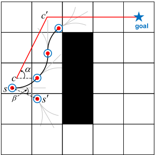
In the 3D search phase, for the currently expanded 3D \( [\begin{matrix}x & y & ψ \\ \end{matrix}] \) , let planner search for states, retrieving each subsequent state based on the designed motion primitive. Calculate the angle between the positive x-axis and the vector β from \( {s_{i}} \) to \( {s_{i+1}} \) . If the deviation between α and β is greater than the threshold value ε, assume that the vector from \( {s_{i}} \) to \( {s_{i+1}} \) is in an undesirable search direction, and the corresponding motion primitives do not involve the actual deployment process. However, in the issue discussed in this article, we need to consider the moving subject as a vehicle whose size can be compared to the width of the road, so it is necessary to set a smaller value for ε. Finally, only parts of the designed motion primitives are involved in each expanding process. An approximate schematic diagram is shown in figure 1.
According to the idea presented by the CMU team in the publicly available source code "LocalPlanner. cpp" on Git, the local path planner can receive laser point cloud information after ground segmentation, and then crop the point cloud information, retaining only the point cloud information near the vehicle. Here, all processed point cloud information has been converted into the vehicle coordinate system. In addition to the point cloud data, the route information generated offline based on the point cloud data is also entered into the local planner. Recalling the reference paths just mentioned, in fact, these offline generated paths can be optimized by pruning strategies mentioned earlier.
|
Figure 1. An illustration of searching. α, β are marked on it. Straight line is a global planning path. Black grids represent obstacles. The paths which are pruned are grey while the preserved path is black. (This image is quoted from [3] and can well describe various search paths.) |
3.2.2. Generation of forward prediction paths offline based on cubic spline interpolation. Firstly, initialize the maximum steering angle θ as well as the step length dγ, determine the initial path points, and gives the radius length of the path to search for once γ. Next, let
\( γ={[\begin{matrix}\begin{matrix}0 & dγ \\ \end{matrix} & \begin{matrix}2dγ & ⋯ \\ \end{matrix} & \begin{matrix}γ-dγ & γ \\ \end{matrix} \\ \end{matrix}]^{T}} \) (1)
\( θ={[\begin{matrix}\begin{matrix}0 & {θ_{1}} \\ \end{matrix} & \begin{matrix}⋯ & {θ_{i}} \\ \end{matrix} & \begin{matrix}⋯ & θ \\ \end{matrix} \\ \end{matrix}]^{T}} \) (2)
Here, \( γ \) and \( θ \) are two \( 1*(n+1) \) matrices, where any \( θ \) corresponds to a \( γ \) at the same position with
\( {θ_{i}}=\frac{θ}{γ}*{γ_{i}} (i=0,1,2…n) \) (3)
A matrix is now used to represent the lattice position segments that characterize local path characteristics:
\( x=[{\begin{matrix}\begin{matrix}x_{1}^{T} & x_{2}^{T} \\ \end{matrix} & \begin{matrix}⋯ & x_{i}^{T} \\ \end{matrix} & \begin{matrix}⋯ & x_{n}^{T}] \\ \end{matrix} \\ \end{matrix}^{T}} \) (4)
\( {x_{i}}={[\begin{matrix}{x_{i}} & {y_{i}} & {z_{i}} \\ \end{matrix}]^{T}} \) (5)
Now, a smooth path for forward prediction can be generated with Equations 1-3, whose path points collection can be described as \( {x_{i}}={γ_{i}}*cos{{θ_{i}}} \) and \( {y_{i}}={γ_{i}}*sin{{θ_{i}}} \) .And,“ \( {z_{i}} \) ”can be abandoned, however, it makes sense when \( {z_{i}}=μ{β^{ \prime }} \) (here \( {β^{ \prime }} \) refers to the direction of vehicle movement, μ is an adjustable coefficient). This can further describe the posture of the vehicle, and the information can support the calculation of the cost function based on the car dynamics model, which is mentioned in [20], making the quality of the trajectory higher. Or, it allows the algorithm to be used in 3D space. By the way, a set of path groups can be obtained by iterating through different angle values and nesting search scales. Additionally, a pruning strategy can be used to optimize its search space.
3.3. Path selecting method and comparison
3.3.1. Path selecting method in this article. Under the condition of real-time collection and construction of a dataset of environmental obstacle voxel points using LiDAR, this article applies a method which allows searching obstacle points near or on the path. Based on it, the optimal path, which is a smooth, short, and safe path for vehicles, will be picked out quickly, and the valueless paths will be cut at once. The steps are as follows:
1) Build voxel grids near the path considering the searching radius, which is caused by the blocking effect of the vehicle itself. After generating voxel grids, each grid and path index is calculated offline. By searching for neighbors within a specified distance around a path point in the path set, which belongs to a set of voxel grids, the index relationship table between each voxel grid and the path to be occluded is obtained.
2) Convert the coordinates of the voxel grid generated in the previous step, the previously generated set of path points and the goal point into the coordinates in the vehicle coordinate system. And initialize the value of the range of voxel points sampled by the computer.
3) Then, based on the possible steering of the vehicle body, the voxel points are converted to the corresponding coordinate system of car itself. Because the index relationship between the voxel mesh and the path is already saved when generating the path and voxel mesh, only the ID number of the mesh needs to be calculated to determine which paths will be occluded. Then, it will be pruned.
4) Finally, based on a given weighting function, traverse each path to obtain the optimal path.
3.3.2. Path selecting method in [3]. In [4], Considering the smoothness of local paths and obstacle avoidance constraints, a weighted optimization objective function is defined as
\( f(x)={w_{s}}\sum _{i=2}^{n-1}{[Δ{x_{i+1}}-Δ{x_{i}}]^{T}}*[Δ{x_{i+1}}-Δ{x_{i}}]+\sum _{i=1}^{n}{w_{o}}f_{o}^{2}({x_{i}}) \) (6)
where \( {f_{o}} \) is defined as
\( {f_{o}}({x_{i}})=\begin{cases} \begin{array}{c} {ⅆ_{S}}-τ({x_{i}}) (τ({x_{i}})≤d) \\ 0(τ({x_{i}}) \gt d) \end{array} \end{cases} \) (7)
And what the method in [2] want to find is the path \( {x^{*}} \) defined as
\( {x^{*}}=\underset{x}{argmin}{f(x)} \) (8)
The obstacle avoidance constraint-solving module is configured to calculate the continuously differentiable distance function \( τ({x_{i}}) \) from the robot to the nearest obstacle based on the Euclidean distance grid map and bilinear interpolation method, and obtain the obstacle avoidance constraint conditions based on the given safe distance from the robot to the obstacle [3].
Using the sparse banded matrix data structure for processing, and refer to the forward elimination and back substitution algorithm to obtain a set of optimal paths. It should be noted that preset initial values and step sizes have a significant impact on the efficiency of the algorithm.
3.3.3. Advantages and disadvantages. The method used in [3] has good computational speed in theory, but in some cases, finding an ideal initial value is not easy. And it decouples map updates from local optimization steps, making its ability to quickly respond to changes mismatched with its computational speed. The method adopted in this paper constantly updates the point cloud information and forward prediction path while the vehicle is moving, making it more resilient.
4. Result and discussion
4.1. Experiment
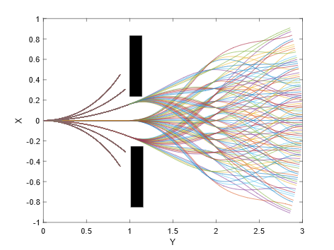
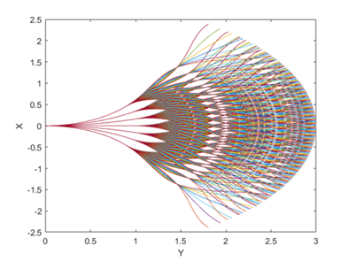
In order to test the effectiveness of pruning strategies for forward prediction paths, comparative experiments were conducted using MATLAB 2022b in the article. In the case of a path search radius of 1, set the scaling reduction parameter to 0.6, use three-layer nesting, set the maximum turning angle to 27°, step size to 0.01, and turn angle traversal step size to 9 °. The pruning condition is simplified to determine the range of steering angles in a known environment, and the relationship between voxels of obstacles and paths is given. In practice, other judgment criteria can be used, such as the nearest obstacle object's mesh angle, etc. If sharp corners are encountered, the use of pruning strategies is meaningful. Moreover, in actual operation, the forward prediction curve that is closer to the original velocity direction angle will be calculated faster, which further demonstrates the rationality of the pruning strategy. Although, in fact, the forward prediction path is generally not nested three times, it may be adopted when the vehicle is moving at high speeds. The increased nesting times in this article is to demonstrate the effectiveness of pruning strategies. The specific experimental results are shown in figure 2 (on the left) and figure 3 (on the right). Note that in figure 3, judgement part will be done in selecting part, so the cost of judgement can be ignored. In theory, the more path branches are pruned, the shorter the time interval for algorithm updates within the same search range. However, the case of pruning a large number of path branches occurs when turning or crossing obstacles, and the update frequency of the algorithm is crucial in these situations.
|
|
Figure 2. An illustration of forward prediction path generation using pruning strategy. The obstacle is painted with black color. It costs 0.139s to judge, prune and generate paths. And the generation part cost about 0.091s. | Figure 3. An illustration of forward prediction path generation mentioned above without judgement. Every curve stands for a path. It costs about 0.161s. |
4.2. Comparison and analysis
In the experiment of [4], it takes 62.83s for the E3Mop Algorithm to lead the robot to the goal point and it travels 44.2m, and in an experiment in [23], it takes about 1458s to travel 886m. The former has a distance to time ratio of approximately 0.703, while the latter has a distance to time ratio of approximately 0.608. It should be noted that the former method [4] has an ideal path data update frequency of 10Hz for DW robot. But the latter [23] can find a feasible short path within only 0.3ms. Even though the latter may not have high path quality and probably requires a significant amount of computing resources during vehicle travel, this ultra-high update frequency is crucial for fast and bulky vehicles. Based on the premise of ensuring collision free and smooth generation, it is essential to try to increase the update frequency as much as possible, generate a certain length of path to guide the vehicle's driving, and strive for calculation time. The reason why it is necessary to increase the update frequency as much as possible is because the driving environment the vehicle is facing is complex and rapidly changing, and collision free is the highest priority requirement. In this process, the length of the generated path, which is the radius of the path search range mentioned earlier, plays a key role. On the one hand, if the path is too short, the prediction of vehicle travel is not comprehensive enough. On the other hand, if the path is too long, the calculation time of the vehicle during the travel process is wasted, and the quality of the path cannot be guaranteed. In addition, the feasibility and efficiency of the algorithm are more crucial, as they directly affect the quality of the generated path and also affect the length of the generated path.
5. Conclusion
This article mainly studies and introduces two path planning ideas for autonomous navigation path planning, namely, pruning strategy and forward path prediction strategy, as well as the idea of constructing maps and selecting routes. And compared the difference between this route selection method based on two strategies and a path selection and generation algorithm in the field of mobile robots. In the experimental section, this article pruned and optimized a forward prediction path generation algorithm proposed by the CMU team based on the pruning strategy mentioned earlier, which improved the efficiency by 13.7% and discussed the possibility of optimization. Note that the efficiency improvement here is conditional. It may not be efficient to deal with complex pruning strategies in high-dimensional motion planning, but it is feasible to intercept a plane for analysis, because the necessary condition for generating a feasible route in space is that the generated path is valid on a plane. So applying the strategies mentioned above to local planning algorithms might improve security level when dealing with complex dynamic motion environments.
References
[1]. Chen J, Xie Z and Dames P 2022 The semantic PHD filter for multi-class target tracking: From theory to practice Robotics and Autonomous Systems 149 103947.
[2]. Chen J and Dames P 2022 Multi-class target tracking using the semantic phd filter In Robotics Research: The 19th International Symposium ISRR p 526-541.
[3]. Wen J, Zhang X, Gao H, Yuan J and Fang Y 2022 E3MoP: efficient motion planning based on heuristic-guided motion primitives pruning and path optimization with sparse-banded structure IEEE Transactions on Automation Science and Engineering 19 2762-2775.
[4]. Wang Y, Cheng W, Li S, Cui X and Su B 2020 Integrated design of local trajectory planning and tracking control for autonomous driving International Conference on Unmanned Systems (ICUS) 1114-1120.
[5]. Wang Q, Su K and Cao D 2019 Path planning for on-road autonomous driving with concentrated iterative search 2019 IEEE Intelligent Transportation Systems Conference (ITSC) 2722-2727.
[6]. Likhachev M, Ferguson D, Gordon G, Stentz A, and Thrun S 2005 Anytime dynamic A: An anytime, replanning algorithm Proc. Int. Consortium Antihypertensive Pharmacogenomics Stud. (ICAPS) 262–271.
[7]. Fox D, Burgard W and Thrun S 1997 The dynamic window approach to collision avoidance IEEE Robot. Autom. Mag. 4 23–33.
[8]. Zhang X, Wang J, Fang Y, and Yuan J 2019 Multilevel humanlike motion planning for mobile robots in complex indoor environments IEEE Trans. Autom. Sci. Eng. 16 1244–1258.
[9]. Treiber M, Hennecke A and Helbing D 2000 Congested traffic states in empirical observations and microscopic simulations Physical Review E 62 1805.
[10]. Zhang L, Ding W, Chen J and Shen S 2020 Efficient Uncertainty-aware Decision-making for Automated Driving Using Guided Branching IEEE International Conference on Robotics and Automation (ICRA) 3291-3297.
[11]. Hubmann C, Schulz J, Becker M, Althoff D and Stiller C 2018 Automated driving in uncertain environments: planning with interaction and uncertain maneuver prediction IEEE Transactions on Intelligent Vehicles 3 5-17.
[12]. Hubmann C, Aeberhard M, and Stiller C 2016 A generic driving strategy for urban environments IEEE International Conference on Intelligent Transportation Systems (ITSC) 1010–1016.
[13]. Speidel O, Ruof J and Dietmayer K 2021 Graph-based motion planning for automated vehicles using multi-model branching and admissible heuristics IEEE International Conference on Autonomous Systems (ICAS) pp. 1-5.
[14]. Zhan W, Chen J, Chan C, Liu C and Tomizuka M 2017 Spatially-partitioned environmental representation and planning architecture for on-road autonomous driving IEEE Intelligent Vehicles Symposium (IV) 632-639.
[15]. Ward E and Folkesson J 2018 Towards risk minimizing trajectory planning in on-road scenarios IEEE Intelligent Vehicles Symposium (IV) 490-497.
[16]. Speidel O, Graf M, Phan-Huu T and Dietmayer K 2019 Towards courteous behavior and trajectory planning for automated driving IEEE Intelligent Transportation Systems Conference (ITSC) 3142-3148.
[17]. Ziegler J and Stiller C 2009 Spatiotemporal state lattices for fast trajectory planning in dynamic on-road driving scenarios Intelligent Robots and Systems IROS IEEE/RSJ International Conference 1879–1884.
[18]. McNaughton M, Urmson C and Dolan J M 2011 Motion planning for autonomous driving with a conformal spatiotemporal lattice IEEE International Conference on Robotics and Automation 4889-4895.
[19]. Gu T, Atwood J, Dong C, Dolan J M and Lee J-W 2015 Tunable and stable real-time trajectory planning for urban autonomous driving IEEE/RSJ International Conference on Intelligent Robots and Systems (IROS) 250-256.
[20]. Likhachev M and Ferguson D 2009 Planning long dynamically feasible maneuvers for autonomous vehicles Int. J. Robot. Res. 28 933–945.
[21]. Samson C 1995 Control of chained systems application to path following and time-varying point-stabilization of mobile robots IEEE Trans. on Automatic Control 40 64–77.
[22]. Gao H, Zhang X, Fang Y, and Yuan J 2018 A line segment extraction algorithm using laser data based on seeded region growing Int. J. Adv. Robot. Syst. 15 1–10.
[23]. Cao C, Zhu H, Yang F, Xia Y, Choset H, Oh J, Zhang J 2022 Autonomous exploration development environment and the planning algorithms International Conference on Robotics and Automation (ICRA) 8921-8928.
Cite this article
Fu,X. (2023). Local planning for autonomous navigation based on forward prediction and motion primitives pruning. Applied and Computational Engineering,10,29-36.
Data availability
The datasets used and/or analyzed during the current study will be available from the authors upon reasonable request.
Disclaimer/Publisher's Note
The statements, opinions and data contained in all publications are solely those of the individual author(s) and contributor(s) and not of EWA Publishing and/or the editor(s). EWA Publishing and/or the editor(s) disclaim responsibility for any injury to people or property resulting from any ideas, methods, instructions or products referred to in the content.
About volume
Volume title: Proceedings of the 2023 International Conference on Mechatronics and Smart Systems
© 2024 by the author(s). Licensee EWA Publishing, Oxford, UK. This article is an open access article distributed under the terms and
conditions of the Creative Commons Attribution (CC BY) license. Authors who
publish this series agree to the following terms:
1. Authors retain copyright and grant the series right of first publication with the work simultaneously licensed under a Creative Commons
Attribution License that allows others to share the work with an acknowledgment of the work's authorship and initial publication in this
series.
2. Authors are able to enter into separate, additional contractual arrangements for the non-exclusive distribution of the series's published
version of the work (e.g., post it to an institutional repository or publish it in a book), with an acknowledgment of its initial
publication in this series.
3. Authors are permitted and encouraged to post their work online (e.g., in institutional repositories or on their website) prior to and
during the submission process, as it can lead to productive exchanges, as well as earlier and greater citation of published work (See
Open access policy for details).
References
[1]. Chen J, Xie Z and Dames P 2022 The semantic PHD filter for multi-class target tracking: From theory to practice Robotics and Autonomous Systems 149 103947.
[2]. Chen J and Dames P 2022 Multi-class target tracking using the semantic phd filter In Robotics Research: The 19th International Symposium ISRR p 526-541.
[3]. Wen J, Zhang X, Gao H, Yuan J and Fang Y 2022 E3MoP: efficient motion planning based on heuristic-guided motion primitives pruning and path optimization with sparse-banded structure IEEE Transactions on Automation Science and Engineering 19 2762-2775.
[4]. Wang Y, Cheng W, Li S, Cui X and Su B 2020 Integrated design of local trajectory planning and tracking control for autonomous driving International Conference on Unmanned Systems (ICUS) 1114-1120.
[5]. Wang Q, Su K and Cao D 2019 Path planning for on-road autonomous driving with concentrated iterative search 2019 IEEE Intelligent Transportation Systems Conference (ITSC) 2722-2727.
[6]. Likhachev M, Ferguson D, Gordon G, Stentz A, and Thrun S 2005 Anytime dynamic A: An anytime, replanning algorithm Proc. Int. Consortium Antihypertensive Pharmacogenomics Stud. (ICAPS) 262–271.
[7]. Fox D, Burgard W and Thrun S 1997 The dynamic window approach to collision avoidance IEEE Robot. Autom. Mag. 4 23–33.
[8]. Zhang X, Wang J, Fang Y, and Yuan J 2019 Multilevel humanlike motion planning for mobile robots in complex indoor environments IEEE Trans. Autom. Sci. Eng. 16 1244–1258.
[9]. Treiber M, Hennecke A and Helbing D 2000 Congested traffic states in empirical observations and microscopic simulations Physical Review E 62 1805.
[10]. Zhang L, Ding W, Chen J and Shen S 2020 Efficient Uncertainty-aware Decision-making for Automated Driving Using Guided Branching IEEE International Conference on Robotics and Automation (ICRA) 3291-3297.
[11]. Hubmann C, Schulz J, Becker M, Althoff D and Stiller C 2018 Automated driving in uncertain environments: planning with interaction and uncertain maneuver prediction IEEE Transactions on Intelligent Vehicles 3 5-17.
[12]. Hubmann C, Aeberhard M, and Stiller C 2016 A generic driving strategy for urban environments IEEE International Conference on Intelligent Transportation Systems (ITSC) 1010–1016.
[13]. Speidel O, Ruof J and Dietmayer K 2021 Graph-based motion planning for automated vehicles using multi-model branching and admissible heuristics IEEE International Conference on Autonomous Systems (ICAS) pp. 1-5.
[14]. Zhan W, Chen J, Chan C, Liu C and Tomizuka M 2017 Spatially-partitioned environmental representation and planning architecture for on-road autonomous driving IEEE Intelligent Vehicles Symposium (IV) 632-639.
[15]. Ward E and Folkesson J 2018 Towards risk minimizing trajectory planning in on-road scenarios IEEE Intelligent Vehicles Symposium (IV) 490-497.
[16]. Speidel O, Graf M, Phan-Huu T and Dietmayer K 2019 Towards courteous behavior and trajectory planning for automated driving IEEE Intelligent Transportation Systems Conference (ITSC) 3142-3148.
[17]. Ziegler J and Stiller C 2009 Spatiotemporal state lattices for fast trajectory planning in dynamic on-road driving scenarios Intelligent Robots and Systems IROS IEEE/RSJ International Conference 1879–1884.
[18]. McNaughton M, Urmson C and Dolan J M 2011 Motion planning for autonomous driving with a conformal spatiotemporal lattice IEEE International Conference on Robotics and Automation 4889-4895.
[19]. Gu T, Atwood J, Dong C, Dolan J M and Lee J-W 2015 Tunable and stable real-time trajectory planning for urban autonomous driving IEEE/RSJ International Conference on Intelligent Robots and Systems (IROS) 250-256.
[20]. Likhachev M and Ferguson D 2009 Planning long dynamically feasible maneuvers for autonomous vehicles Int. J. Robot. Res. 28 933–945.
[21]. Samson C 1995 Control of chained systems application to path following and time-varying point-stabilization of mobile robots IEEE Trans. on Automatic Control 40 64–77.
[22]. Gao H, Zhang X, Fang Y, and Yuan J 2018 A line segment extraction algorithm using laser data based on seeded region growing Int. J. Adv. Robot. Syst. 15 1–10.
[23]. Cao C, Zhu H, Yang F, Xia Y, Choset H, Oh J, Zhang J 2022 Autonomous exploration development environment and the planning algorithms International Conference on Robotics and Automation (ICRA) 8921-8928.