1. Introduction

Housing price is one of the most important topics of society since the demand for residential properties has increased dramatically in the last century because of the surge in population growth rate and higher economic development. One of the phenomena in the housing market is that the prices of residential properties can vary considerably, although they are in the same city or province. It is important to figure out what factors can make this difference in housing prices because this can be used as a guide for future city planning and residential property construction to meet citizens’ demands better.

This paper focuses on the relationship between regional median housing prices and some characteristics of the region, such as population and average income. A multiple linear regression (MLR) model will be constructed in this essay for market price prediction and to select the most influential factors that can affect housing prices for residential properties in different districts of California.

The research on housing prices supports the hypothesis that real prices of residential properties have a positive correlation with the real incomes in a region by using a spatial-temporal model [1-2]. It has also been found that the age of the apartment is negatively correlated with its market price, in both global and local regression models [3]. Population density has a positive correlation with housing prices, as found by regional regression in 285 Chinese cities [4]. Apart from the factors verified by these researchers, the number of households and the total number of rooms will also be included in this model as regressors since differences in family sizes can result in varied evaluations of property prices.

R will be used to construct different MLR models with different regressors and make a comparison between them to select the one with the greatest explaining power and the smallest variance inflation factor (VIF). The selection process will be described in the section on model development. The final model will contain the most significant regressors and their beta coefficients to show how one unit change in those factors will affect the regional housing price.

2. Exploratory Data Analysis

2.1. Data Resource

The data set used for this essay is loaded from Kaggle, containing 20433 entries of data for the housing market in California, with 10 categories of information. After omitting all the null values, 500 rows from this dataset would be selected and divided into test data and training data randomly to develop the MLR model.

2.2. Description of Data

Table 1: Comparison between Train and Test Dataset for Numerical Categories

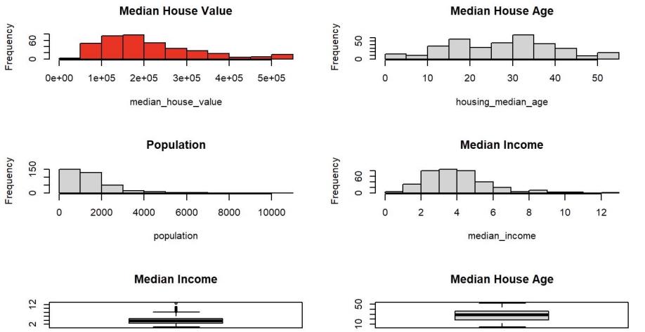
Figure 1: Histograms and Boxplots for Important Data

Characteristic information such as minimum, maximum, median, and mean values of the numerical category have been summarized in Table 1. It can be seen from Table 1 that the mean and the quantiles of both the train and test datasets are very close; this is because both are randomly selected from the original large dataset to make the result from model construction from the training dataset more general and can be applied on the test dataset for the final result.

Figure 1 presents four histograms and two boxplots for the important numerical data, including the response value (average housing prices), and the regressors that will be used in the model. It can be seen from the graph that the median housing value and the median income are more normally distributed than the median housing age and population. However, it can be seen from the box plots that there are more large outliers in median income than in the median housing age, and the disparity of average income is overall smaller than the median age. It is noticeable that the unit of the median income is in thousand dollars.

2.3. Testing the Important Predictors for Correlations

The scatter plots with the best-fit lines of median house value with respect to median house age and median income respectively are plotted to investigate the correlations between them. From Figure 2, it is obvious that both correlations are positive, but the median income has a stronger correlation with the median housing value than the median housing age because the points in the right graph are much closer to the best-fit line; both are acceptable to be added to the first model.

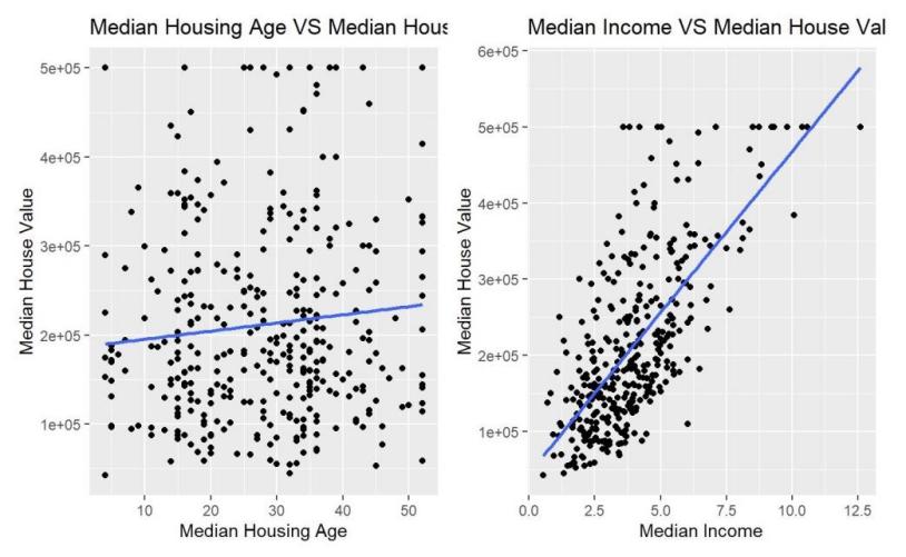
Figure 2: Scatter Plots of the Median House Value with respect to Median Housing Age and Median Income Respectively

3. Model Development

3.1. Model Construction Process and Selection

Table 2: Final Results and Indicators of the Four Models

By using the predictors introduced before, R will be used to generate Model 1 by multiple linear regression of median housing price on median housing age, population, number of households, median income, and the total number of rooms. The result shows that the p-value of the total number of rooms is 0.182, which is larger than the 0.05 significance level, which means the hypothesis for the coefficient in front of it to be zero is supported; so this predictor should be removed and the next step is to try a new regression for the same responsory on the other four predictors, and this is the model 2. The result shows that all four predictors in Model 2 have less than 0.05 p-values, which means all of them are significant predictors.

After that, predictor population is removed from Model 2 to construct Model 3 and conduct a partial F test to find out which of them is better. This is because the predictor population may cause multicollinearity issues with the household predictor. After conducting the test, the p-value is 3.413e-10, which is smaller than the 0.05 significant level, so Model 2 is a better model. After conducting a stepwise selection by R, the result shows Model 2 has the smallest Akaike information criterion(AIC) of all the models; therefore, Model 2 is chosen to be the final model here. As shown in Table 2, the mean VIF of Model 2 is less than 5, so there is no multicollinearity problem in Model 2.

3.2. Apply Final Model on Test Dataset

After selecting the final model to be Model 2, it will be applied on the test dataset to find out whether the model is generalized for all datasets. The model using the regression form of Model 2 and the test dataset is Model 4; As shown in Table 2, the explaining power of Model 4 is the greatest, and the mean VIF is also smaller than 5, so there does not exist multicollinearity issues in Model 4 [5].

From Table 2, it can be seen that the correlations between the four predictors and the median housing price stay on the same sign, and the coefficients in front of them are close. Therefore, Model 2 is generalizable to the test dataset, and Model 4 can be used for conclusion if all assumptions are satisfied.

3.3. Model Diagnostics

In this section, it is aims to find out if Model 2 and Model 4 satisfy the assumptions of multiple linear regression by using the method from the book “A Modern Approach to Regression with R” [6]. All four graphs are very similar for both models.

Firstly, as shown in Figure 3 and Figure 4 below, the residuals of both models fit the line well, so the residuals of Model 2 and Model 4 are normally distributed. For the residual plots, there are no distinct patterns for residuals spreading around the horizontal line, and there are no clusters or fanning patterns in the plot. Therefore, linearity and independence are also satisfied. For the Scale-Location plots, points are spread equally with a horizontal line, so the constant variance is also satisfied for both models.

From the residual versus leverage plots, although there are more influential points in Model 2 than in Model 4, there is no reason for them to be removed.

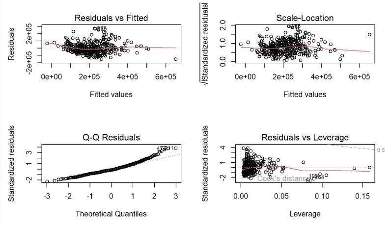
Figure 3: Plots for Model 2 Diagnosis

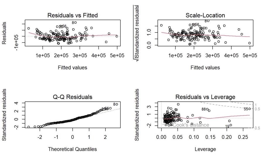
Figure 4: Plots for Model 3 Diagnosis

4. Conclusion

This paper aims to find out the most influential factors for the regional housing price in California by using the method of MLR. From the analysis above, the final model produces very close outputs using both the training dataset and the testing dataset. Therefore, it is reasonable to accept the interpretations from Model 3 for the relationships between influential factors and housing price itself.

Based on the result in Table 2, the interpretation can be seen as keeping all other factors unchanged, one unit change in median income, median housing age, households, or population will result in 45309, 2460.26,190.80, -53.77 units of change in regional median housing price respectively.

Therefore, if the government wants to lower the housing price for one region, it can build more residential properties there to decrease the median housing age. This policy works because supply changes faster than demand in this case and lowers the regional housing prices. With all other factors unchanged, when people are considering where they are going to purchase a residential property, they can compare their income with the regional median income for more rational decisions.

However, there remain limitations to this MLR research. Firstly, the total area of each district is unknown in this dataset, so the population density is unknown, and population and the number of households are used instead. This may lead to multicollinearity when the model is applied to other datasets and leaves the relationship between regional housing prices and population density ambiguous. Moreover, this dataset only contains data from California, so its results may not be generalized to other areas or countries. However, this method of analysis is transferable to other investigations in other areas, such as marketing and social services, as long as the assumptions of MLR are satisfied.

References

[1]. Pace, R. Kelley, and Ronald Barry. "Sparse spatial autoregressions." Statistics & Probability Letters 33.3 (1997): 291-297. https://www.kaggle.com/datasets/camnugent/california-housing-prices
[2]. S. Sisman, A.C. Aydinoglu “A modeling approach with geographically weighted regression methods for determining geographic variation and influencing factors in housing price: A case in Istanbul” https://doi.org/10.1016/j.landusepol.2022.106183
[3]. Sean Hollya, M. Hashem Pesarana, Takashi Yamagata “A spatio-temporal model of house prices in the USA” doi: 10.1016/j.jeconom.2010.03.040Yanchao Feng “Examining the determinants of housing prices and the influence of the spatial–temporal interaction effect: The case of China during 2003–2016” https://doi.org/10.1016/j.cjpre.2021.04.013
[4]. Yanchao Feng “Examining the determinants of housing prices and the influence of the spatial–temporal interaction effect: The case of China during 2003–2016” https://doi.org/10.1016/j.cjpre.2021.04.013
[5]. Noora Shrestha, Detecting Multicollinearity in Regression Analysis, American Journal of Applied Mathematics and Statistics. 2020, 8(2), 39-42. DOI: 10.12691/ajams-8-2-1
[6]. Simon J. Sheather. A Modern Approach to Regression with R. ISBN:978-0-387-09608-7. page 151.
Cite this article
Cao,Y. (2024). Influential Factors on California Regional Housing Price Analysed by Multiple Linear Regression. Advances in Economics, Management and Political Sciences,77,48-53.
Data availability
The datasets used and/or analyzed during the current study will be available from the authors upon reasonable request.
Disclaimer/Publisher's Note
The statements, opinions and data contained in all publications are solely those of the individual author(s) and contributor(s) and not of EWA Publishing and/or the editor(s). EWA Publishing and/or the editor(s) disclaim responsibility for any injury to people or property resulting from any ideas, methods, instructions or products referred to in the content.
About volume
Volume title: Proceedings of the 3rd International Conference on Business and Policy Studies
© 2024 by the author(s). Licensee EWA Publishing, Oxford, UK. This article is an open access article distributed under the terms and
conditions of the Creative Commons Attribution (CC BY) license. Authors who
publish this series agree to the following terms:
1. Authors retain copyright and grant the series right of first publication with the work simultaneously licensed under a Creative Commons
Attribution License that allows others to share the work with an acknowledgment of the work's authorship and initial publication in this
series.
2. Authors are able to enter into separate, additional contractual arrangements for the non-exclusive distribution of the series's published
version of the work (e.g., post it to an institutional repository or publish it in a book), with an acknowledgment of its initial
publication in this series.
3. Authors are permitted and encouraged to post their work online (e.g., in institutional repositories or on their website) prior to and
during the submission process, as it can lead to productive exchanges, as well as earlier and greater citation of published work (See
Open access policy for details).