1. Introduction

Sharing economy is a new business model that depends on online platform. The business develop with the development of digital economy. Richardson defined it as:’ the sharing economy refer to forms of exchange facilitated through online platform, encompassing a diversity of for--profit and nonprofit activities that all broadly aim to open access to under-utilized resources through what is termed sharing.’[]Kuhzady et al. divided the notions of sharing economy into four group and namely: transportation, dining, tour guide services and accommodating.[]It is benefit to economy, Fraiberger et al. develop a dynamic model and study the data form US automobile industry. They uncover that sharing economy will increase the surplus significantly.[]

Airbnb is an online short-term room sharing platform that connects owner to share with those ones who need accommodation. Scholars have study form multiple perspectives in it. scholars exam the effect of Airbnb on the hotel industry and found that it decreases the price of hotels. []Fang et al. shows that the sharing economy creates job position because it decreases the price of hotel and attract tourist. However, the effect decrease with the size of sharing economy increasing because the Airbnb house which do need need to hire employee replace the hotel demand.[] Scholars also study the behavior of supplier and consumers. Edelman et al. uncovered that Airbnb will lead to digital discrimination by studying the Airbnb data from New York City. They show that the non-black hosts will charge more than 12% than black ones. []

The sharing economy has significance on the supply research because it allows people to render service in a flexible and low-cost way based on under-utilized resources. Chen et al. studied the Uber drivers’ data and found that the flexible work will increase the surplus and drivers would work more on the flexible work.[] The determinant of supply of the sharing economy is a topic that scholars focus on. Gutierrez et al. discovered that the hotel supply and tourist attraction have significant correlations with hosting.[] Quattrone et al. analyzed the data of Airbnb from London and found the influence of socioeconomic characteristics on hosting.[] Yang et al.based on Airbnb data in 28 major cities in the US analyzed the influence of tourism, hotel supply, regulation, and status of residential and owner and uncover that certain regulations may complicate the hosting.[]

However, the vast majority of literature focuses on the economic environment and does not uncover the influence of the status of the owner and unit on the market performance and accommodating supply. Our work will research it from a micro perspective.

2. Data source and summary

We get a data set about the properties in New York City from Airbnb. To control the effect of location, all of the properties are distributed in southeastern Manhattan as Figure1 shows. The data set includes 2331 properties information in New York City. Table1 shows a summary of the data. Figure2 shows the correlation among each variable.

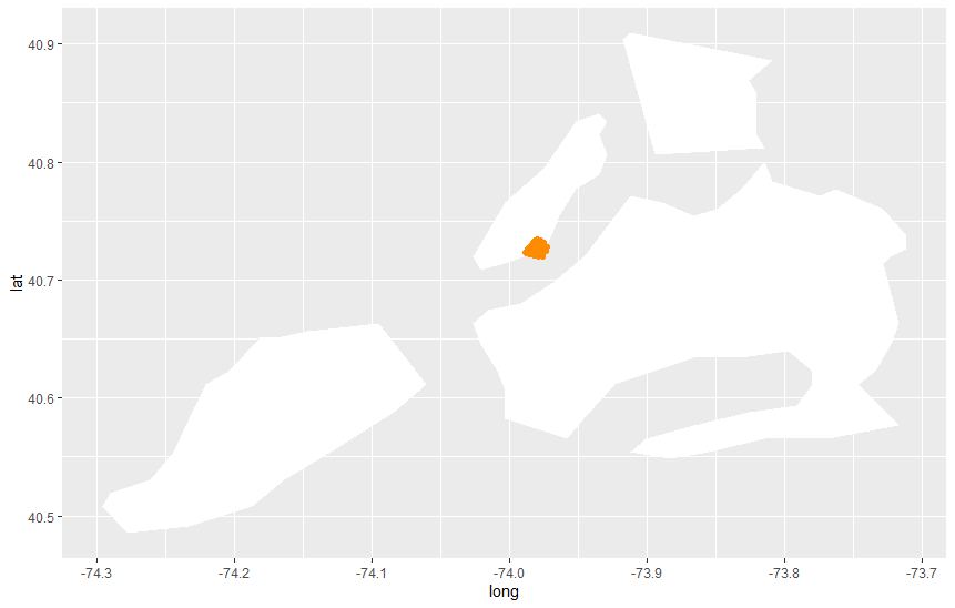
Figure 1: Distribution of properties.

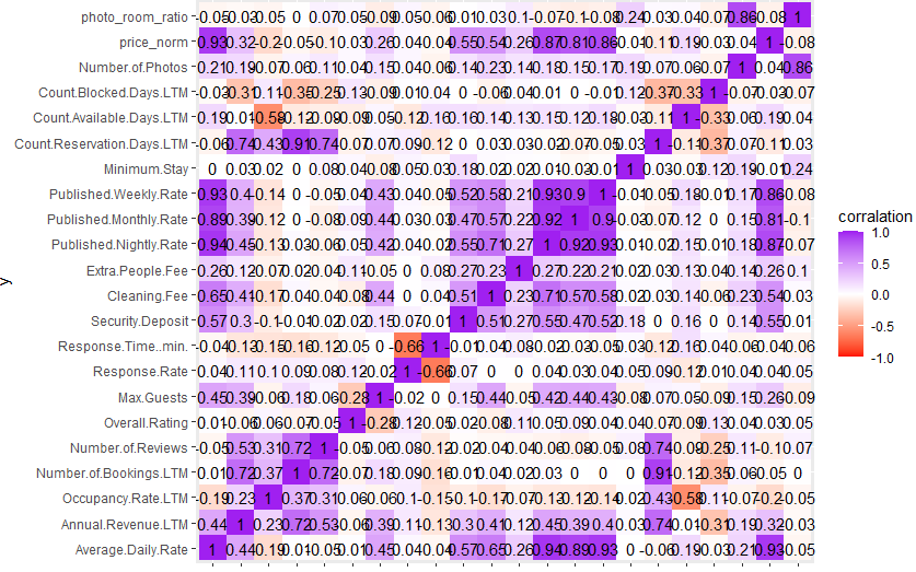
Figure 2: Correlation coefficient between variables.

Table 1: Summary of data.

There is some difference among the properties on Airbnb. The sample is divided by household types and listing types.The distribution is shown in Table2. It is obvious that the apartment is the majority. The reasons might be that southeastern Manhattan has much more apartments than other types of properties and the apartment is the most economical option because the cost is lower and the rental demand has a little difference in different types and is sensible to price. It is obvious that the entire home/apt rate is the majority in the peer-to-peer rental market.

Table 2: Types of samples.

Airbnb will give the hosts the title so-called ‘Superhost’, which will bring more revenues and needs more effort. So we think that the proportion of Superhost will show the hosts’ behaviors and strategies. The distribution is shown in Figure3. It shows that only 6% of hosts become Superhost.

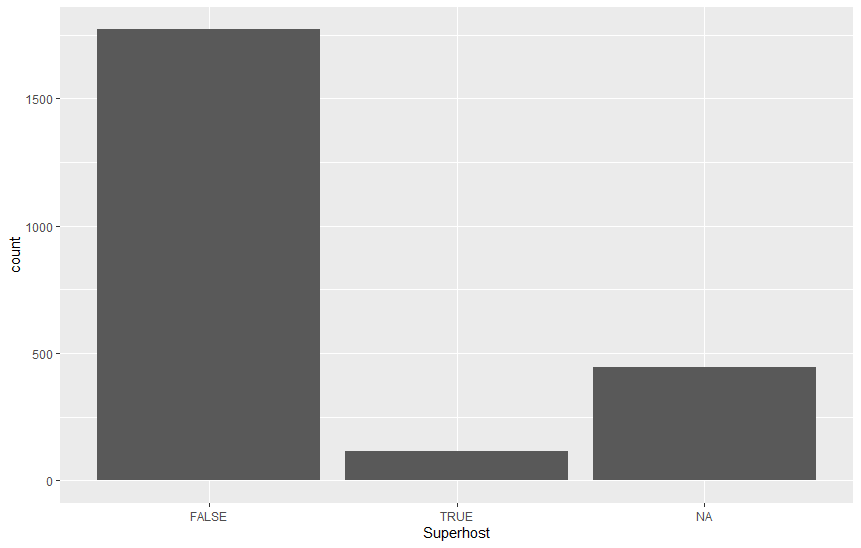
Figure 3: structure of hosts.

3. Empirical analysis

3.1. How do statues affect market performers

We consider the status of the properties as the factor that will affect the market performers.

We test the majority of variables for each type of property type and listing type. The results are shown in Table 3 and Table 4. They show that the properties’ type affects the income and price. The higher quality type would lead to higher prices and more revenues. And the Occupy rate has less relation with the properties type.

The listing type also makes a difference in the performance. The entire home has higher daily rates, more revenues, and more occupancy rates.

Table 3: summary of each properties' types.

Table 4: summary of each listing type.

To understand the effect of title “superhost” we show the mean values of average daily rate, annual revenue, and occupy rate in Table5. It shows that the superhost will get more revenue from Airbnb.

Table 5: summary of superhost and non-superhost.

We do line regression to figure out the effect of the valuables. We fill the NA value with average value and winsorize upper and lower 1% to eliminate the effect of outlier.

Table 6: regression result of number of bookings.

We do regression and test the effects on the number of bookings. The result is shown in Table1. It shows that more information such as Instantbook and photos will increase the number of bookings, which indicates that the consumers highlight the shopping experience. They prefer to have more information about services and would like to decrease the time cost. What’s more, it is wired that the rate and demand have a positive relation. It might have 2 reasons. First, the quality of properties in the platform varies in a large range and consumers are more sensitive to the quality than price. Second, consumers lack information, so they will assume that the higher price means the higher quality. We also find that the additional fees do not have significant effect on the a number of bookings of entire home/apt. But it has significant negative effects on the private home. Plus, we also notice that almost all the factors show insignificant effect on shared room. We report the test graph of the regression in Figure

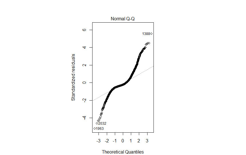
Figure 4: Normal Q-Q.

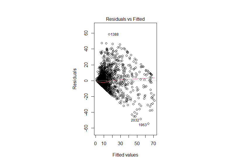
Figure 5: Residual vs Fitted values.

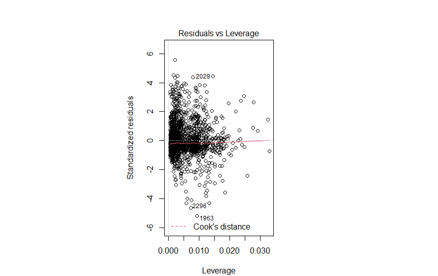
Figure 6: Residuals vs Leverage.

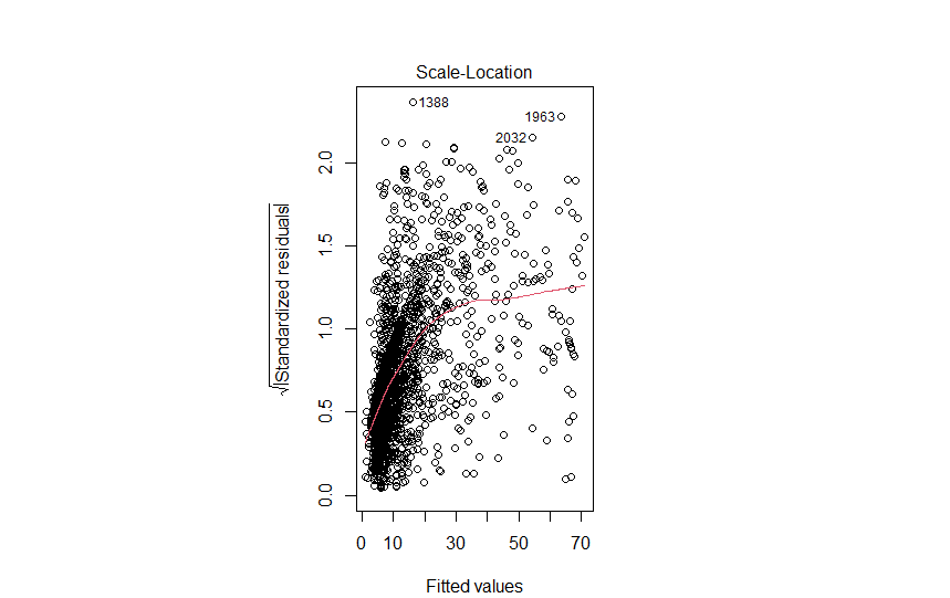
Figure 7: Scale-Location.

We also do regressions to test the effect of each variable on annual revenue. The result is shown in Table2. It shows that the rooms of properties will affect the annual revenue. The information also can have positive effect because it will create the trust and decrease the risk. published nightly rate and clean fee have a positive effect on the revenue. We report the test graphs in Figure.

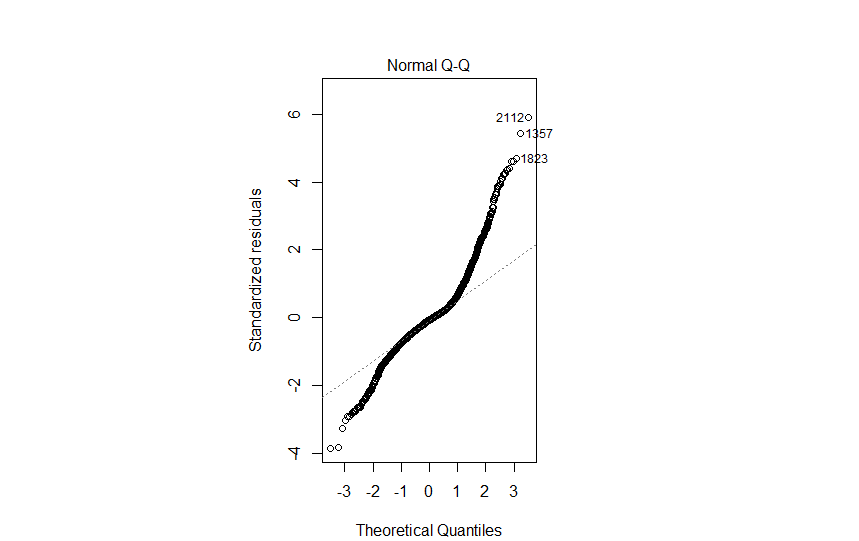
Figure 8: Normal Q-Q.

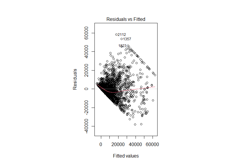
Figure 9: Residuals vs Fitted values.

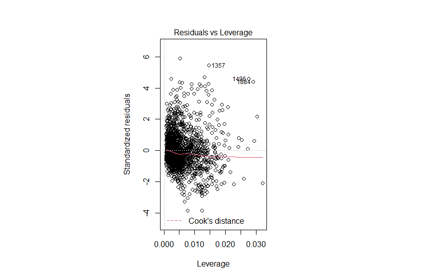
Figure 10: Residual vs Leverage.

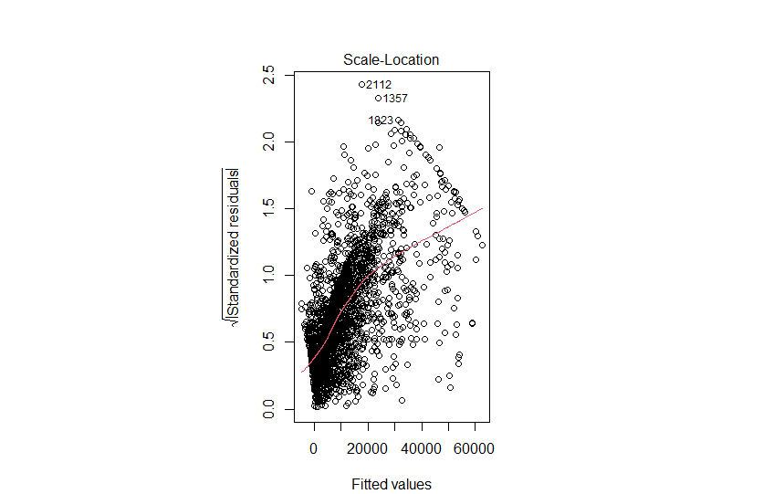
Figure 11: Scale-Location.

Table 7: Regression result for annual revenue.

3.2. The host providing behavior

For each property, the daily status file has A, B, R as available, block, and occupied status of the property. and we show the effect of the host and properties on the status.

We have a Markov transition matrix to show the transition process. The matrix is shown in Table8. We can tell some characteristics of it. First, the hosts would like to stay in the same state for some time. Second, the steady states are shown in Table9, which shows that hosts have the same probability in the 3 statuses.

Table 8: Markov Transition matrix.

Table 9: Steady State.

To understand the behavior of block, we do a survival analysis of the time between blocks. We analyze the data of April 2016 for the properties. and the results are shown in Table 6 and Figure 4.

Table 10: result of survival analysis.

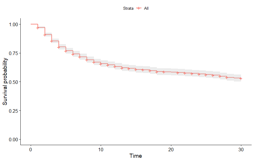
Figure 12: survival analysis.

It shows that most hosts would not change to block in a month. Besides, the slope of the curve slopes after 15 days. This change might show a part of the hosts’ behaviors that they would like to have a break in a half month. We also do the survival analysis for each listing type. The results are shown in Figure 5. It shows that the entire home/apt is more likely to choose blocks. Combining it with the result of descriptive statistics for each listing type, it might shows that the better performers would lead to more breaks.

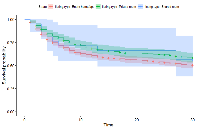
Figure 13: survival analysis for each listing type.

We build a logistical regression model to test the effect of determinants on the block inclination and show the result in Table1 and Table2.

As we show in the Markov matrix, the behavior is constant. Last A and Last R will decrease the probability of block. A and R will show the owners short-term behavior and revenue.

The expected occupied rate would be the determinant of block behavior. Annual revenue Price and R can be a speculative basis for short-term occupancy rates. The higher price will let hosts think that it has the lower possibility of being chosen. Weekend means that there are more tourists. The higher annual revenue and short-term occupied rate also let the host believe that the hosting is catchy in the term. Therefore, they would supply it and have less probability of being blocked.

Shared room is an interesting case in the analysis because it shows lots of differences with others. We guess that leisure plays a more important role in the case. That is the reason Why the number of days occupied, annual revenue, superhost, and price show a significantly positive effect on the block inclination.

Table 11: result of logit model with readom effect.

Table 12: result of logit model.

4. Conclusion

We test the effect of the status on the performance and supply behavior and get our conclusions. First, different listing types lead to different performance and supply behavior. Entire home/apt have the best performance and the supply behavior is similar to the private room. Shared room is different from other types. Second, better service and more information will lead to better performance. Tired, consumers prefer properties with a higher price and additional fees do not affect it. Forth, Leisure and expected occupy rates affect supply behaviors.

Our study has some Limitations. Considering that we just do regression on the number of block days, we do not study the factors’ effect on the frequency of block days that we show in the survival analysis. Besides, it seems that there are different ways the factors affect the Shared room. And we do not find it.

References

[1]. Richardson, L. (2015). Performing the sharing economy. Geoforum, 67, 121-129.
[2]. Kuhzady, S., Seyfi, S. and Béal, L. (2022). Peer-to-peer (P2P) accommodation in the sharing economy: A review. Current Issues in Tourism, 25(19), 3115-3130.
[3]. Fraiberger, S. P. and Sundararajan, A. (2017). Peer-to-peer rental markets in the sharing economy. NYU Stern School of Business Research Paper (First version March 2015.
[4]. Fradkin, A., Grewal, E. and Holtz, D. (2018). The determinants of online review informativeness: Evidence from field experiments on Airbnb. SSRN Electronic Journal, 41, 1-12.
[5]. Fang, B., Ye, Q. and Law, R. (2016). Effect of sharing economy on tourism industry employment. Annals of tourism research, 57, 264-267.
[6]. Edelman, B. G. and Luca, M. (2014). Digital discrimination: The case of Airbnb. com. Harvard Business School NOM Unit Working Paper, (14-054).
[7]. Chen, M. K., Rossi, P. E., Chevalier, J. A. and Oehlsen, E. (2019). The value of flexible work: Evidence from Uber drivers. Journal of political economy, 127(6), 2735-2794.
[8]. Gutiérrez, J., García-Palomares, J. C., Romanillos, G. and Salas-Olmedo, M. H. (2017). The eruption of Airbnb in tourist cities: Comparing spatial patterns of hotels and peer-to-peer accommodation in Barcelona. Tourism management, 62, 278-291.
[9]. Quattrone, G., Proserpio, D., Quercia, D., Capra, L. and Musolesi, M. (2016, April). Who benefits from the" sharing" economy of Airbnb?. In Proceedings of the 25th international conference on world wide web (pp. 1385-1394).
[10]. Yang, Y. and Mao, Z. (2019). Welcome to my home! An empirical analysis of Airbnb supply in US cities. Journal of Travel Research, 58(8), 1274-1287.
Cite this article
Zhou,J. (2024). When Would Owners Decide to Block Their Properties? Deciphering the Airbnb Business Decisions with Transactional Data. Advances in Economics, Management and Political Sciences,79,16-31.
Data availability
The datasets used and/or analyzed during the current study will be available from the authors upon reasonable request.
Disclaimer/Publisher's Note
The statements, opinions and data contained in all publications are solely those of the individual author(s) and contributor(s) and not of EWA Publishing and/or the editor(s). EWA Publishing and/or the editor(s) disclaim responsibility for any injury to people or property resulting from any ideas, methods, instructions or products referred to in the content.
About volume
Volume title: Proceedings of the 3rd International Conference on Business and Policy Studies
© 2024 by the author(s). Licensee EWA Publishing, Oxford, UK. This article is an open access article distributed under the terms and
conditions of the Creative Commons Attribution (CC BY) license. Authors who
publish this series agree to the following terms:
1. Authors retain copyright and grant the series right of first publication with the work simultaneously licensed under a Creative Commons
Attribution License that allows others to share the work with an acknowledgment of the work's authorship and initial publication in this
series.
2. Authors are able to enter into separate, additional contractual arrangements for the non-exclusive distribution of the series's published
version of the work (e.g., post it to an institutional repository or publish it in a book), with an acknowledgment of its initial
publication in this series.
3. Authors are permitted and encouraged to post their work online (e.g., in institutional repositories or on their website) prior to and
during the submission process, as it can lead to productive exchanges, as well as earlier and greater citation of published work (See
Open access policy for details).