1. Introduction

The capital asset pricing model (CAPM) is the relationship between investment risk and expected return for stocks [1]. In the CAPM formula, \( {R_{i}} \) is the rate of return of a given stock, while \( {R_{m}} \) is the rate of return of the market. \( {R_{f}} \) is the risk-free rate of return, a guaranteed return for an investment with zero risk [2]. Usually, the current Treasury bill (T-bill) is used for the risk-free rate. This is because T-bills are backed by the government, therefore having close to zero risk [3]. The beta ( \( ß \) ) value is the sensitivity of a stock to returns on the market, always estimated based on an equity market index [4]. The CAPM formula was chosen for our research because of its simplicity and easily comparable results.

It is important for investors to know the risk level they will be taking on when making any investment decision. In our research, we focused on the investment of stocks, where the risk is largely due to the volatility of the stock. Therefore, it was decided to calculate the beta values of stocks in four different industries, comparing their volatilities to each other and to the market, S&P 500, to see the different risks involved in investing in each of them. The time period was selected because of the recent pandemic, which likely has an effect on the sensitivities of the stocks. The purpose of this article is to see the effects of the COVID pandemic on the sensitivities of different industries, or how COVID could have impacted their beta values.

2. Literature Review

The financial study of beta values of different industries and stocks is important for investment decision-making, allowing investors to gauge the risk and reward of investing in a given stock. This research involves using asset-pricing models, including CAPM, to solve for beta. Analyzing beta values can not only be used for investment decision-making but can also give the researcher insight on different industries and on the current state of the market. CAPM was first proposed by William Sharpe, Jack Treynor, John Lintner and Jan Mossi in the early 1960s.

Over time, there has been debate over the reliability of CAPM for investment decision-making. In the article written by Ante Perković in 2011 [5], research is done using the Croatian market to test beta and the concept of CAPM, to find a correlation between beta and return. The results show that there is no relationship between the beta and return, likely because of the nature of the CAPM formula: that it is only for portfolios and does not include individual securities. However, the opposite result is seen in another article written by Ralf Elsas, Mahmoud El-Shaer, and Erik Theissen in 2003 using the German stock market [6]. They explained their differing results from previous research that found no relationship because the average market risk premium had been close to zero. Despite these differences in results about the reliability of CAPM and of the beta value itself, CAPM is continuously used to measure volatilities of different stocks, sectors, indexes, and industries over time, giving it a certain degree of credibility for current and future research.

In both the papers written by Chris Tofallis [7] and Enny Istanti & Bramastyo Kusumo Negoro [8], linear regression (or line of best fit) is used to find beta values. The type of regression Istanti and Negoro use is multiple linear regression, their results showing that earnings per share and financial leverage have no significant effect on the beta while asset growth does have a significant effect on beta. Tofallis uses a different line fit that is both more reliable and easier to understand to find an “alternate” beta, which his research found to be the equivalent excess rates of returns, corresponding exactly to the relative volatility of an investment, one of the interpretations commonly included with the concept of beta. Similar to Tofallis, in the paper written by Vincent J. Hooper, Kevin Ng, and Jonathan J. Reeves [9], the goal is to lower the error of beta forecasts, finding that the AR(2) model has half the error of that of the constant beta model. These articles show that although CAPM and beta may not be as reliable, there can be great improvements made to the calculation method for both to increase reliability and reduce error, even making calculation easier than before.

Jiawei Hong, Xiaojian Yu, Weilin Xiao, and Xili Zhang [10] used 27 alternate methods for estimating beta in the Chinese stock market, finding negative returns in the portfolio analysis, likely due to the market’s restricted short-selling, leading to the underperformance of stocks in the market. They look to find a way to explain future stock returns. Reza Bradrania, Jose Francisco Veron, and Winston Wu [11] studied the relationship between the beta anomaly and stock quality in international stock markets, finding a statistically significant beta anomaly in low-quality stocks and no beta anomaly in high-quality stocks in both portfolio and regression analyses. Similarly, they look for a relationship between the quality of stocks, the beta anomaly, and the returns of the stocks.

Finally, the paper written by Syed Mohammad Faisal, Ahmad Khalid Khan, and Omar Abdullah Al Aboud [12] looks to find beta in order to create awareness about risk in investment decisions. They also use CAPM to find beta values in the Indian market for infrastructure, healthcare, and software due to the high demands in those three sectors. Our research is most similar to theirs, although we selected four industries rather than only three. Historical data (a time series) was also used for their calculations, although it was a longer series and therefore likely to be more accurate than the results discussed in this paper.

CAPM is a simple and useful equation for getting general ideas of the risks in investing in different industries, although its reliability and accuracy is still open to future research. The beta value itself seems to be under constant research as well, as more and more alternative methods are found and created to find these beta values in a simpler and/or more accurate way than before. The analysis of both the calculation method and the beta values themselves can be highly useful for future investment decisions, reducing individual losses of investors and increasing accuracy of predictions of future returns of a stock or industry.

3. Methodology

3.1. Selection of Market, Risk-Free Rate, and Time Period

The authors chose the S&P 500 Index (Bloomberg ticker: SPX) for calculating \( {R_{m}} \) because it is one of the most representative equity market indices in the US capital market, including the leading companies across different sectors both in and outside the US. The large transaction volume per day, well-diversified institutional investors, and its long history indicate that the market should be relatively close to the market with efficient market assumption in CAPM model theory. The return of SPX could be a reference benchmark during comparison of specific sectors.

The authors chose the 1-year T-bill for our \( {R_{f}} \) since we are doing research in the US market, and therefore the government bonds issued by the US government should be the most appropriate candidate. In theory, T-bill should be risk-free given its government-backed nature. 1-year was the tenor because our research time period is from January 31, 2022 to December 31, 2022.

The authors selected the year of 2022, where each month would have a calculated beta value. However, to use linear regression, a time series was used stretching back to three years, from 2019 to 2022. For example, if the beta for January 31, 2022 was being calculated, the time series would be from January 31, 2019 to January 31, 2022.

3.2. Selection of Industries and Stocks

The authors selected four industries: transportation banking, retail, and media and entertainment. These four industries were chosen because they are not closely related and therefore will not be largely affected by each other. For example, if consumer spending increases in the retail industry, the media and entertainment industry’s prices are not likely to increase or decrease as a result.

The authors found the data for each industry in Bloomberg and Capital IQ. For transportation and banking, the top 100 companies based on market cap were selected. The selection criteria is based on the Bloomberg Industry Classification System (BICS) Level 2 industry classification standard, as well as the Ratings Direct industry standard (Capital IQ). After the preliminary selection, the ones that went IPO, delisted, or suspended trading in 2022 (therefore lacking the full price data needed to calculate beta) were removed. Table 1 shows the resulting numbers of companies selected in each of the sectors:

Table 1: The chosen industries and number of companies for each industry.

3.3. Single Stock Beta Calculation

In our research, the historical return of single stock \( i \) is calculated by the capital gain of a single stock within a certain period:

\( {R_{i}}={(P_{t}}-{P_{t-1}})/{P_{t-1}} \)

where \( {R_{i}} \) is the rate of return, \( {P_{t}} \) is the price of the current day, and \( {P_{t-1}} \) is the price of the previous day.

As an estimation exercise, monthly frequency was used in this paper to balance the efficiency and accuracy. The price at the end of each month was used to calculate the \( {R_{i}} \) in a single month and annualize the calculated return by multiplying 12. The \( {R_{m}} \) (return rate of the market, SPX) is calculated the same way. Then, each stock’s respective beta values were calculated using the CAPM formula in a spreadsheet. The CAPM formula is stated as:

\( {E(R_{i}})-{R_{f}}={ß_{i}}*(E({R_{m}})-{R_{f}}) \)

Since beta is a description of the elasticity between the extra stock return and the extra market return, the beta is estimated (i.e. the slope of the above formula) by doing regression of extra historical return of a single stock \( i \) ( \( {R_{i}}-{R_{f}} \) ) versus that of the capital market ( \( {R_{m}}-{R_{f}} \) ). This is calculated by linear regression function (i.e. the LINEST function in Microsoft Excel), where the y-value is \( {R_{i}}-{R_{f}} \) , the x-value is \( {R_{m}}-{R_{f}} \) , and the y-intercept is \( 0 \) . The time series was lengthened back to as long as three years (36 data points, one for each month) for the regression. For example, to calculate the beta for one stock in January 2022, linear regression was done between the extra historical return of that stock from January 2019 to January 2022, and that of the capital market over the same period.

3.4. Industry Beta Calculation

Once the beta value was calculated for all stocks over the research period, the weighted beta was calculated using the formula below:

\( {ß_{iw}}=({ß_{i}}*MK{P_{i}})/MK{P_{T}} \) ,

where \( {ß_{iw}} \) is the weighted beta of the stock \( i \) , \( {ß_{i}} \) is the raw beta value of the stock \( i \) , \( MK{P_{i}} \) is the market capital of the stock on the given date, and \( MK{P_{T}} \) is the total market capital of the industry on the given date, calculated by adding the market cap of all stocks in the industry on the given date. Market cap was used to weight the betas because market cap is a measure of what a company is worth in the market, and also a representation of how much a single stock’s price can affect the market price. For example, if the market cap of one stock was 10 and the market cap of another stock was 100, the second stock would affect the market price more than the first stock.

The beta for the entire industry \( k \) for a specific month in 2022 was then calculated by adding the weighted betas of each stock in the respective month:

\( {ß_{k}}=Σ{ß_{i}} \)

4. Results

Based on the methodology described earlier, for each of the industries, there are 12 data points as output. As our research covers four industries, the total number of data points is 48. Table 2 shows the beta values of each month in 2022 of the four industries selected for research. Overall, the media and entertainment industry has the highest beta values, while the retail industry has the lowest beta values.

Table 2: Calculated Beta on Four Industries through 2022 Full Year

Table 3 shows the descriptive statistics for the beta values of the four industries, including the mean and standard error. The mean values of each industry indicate the general sensitivity of the industry’s stocks in 2022, while standard error points to the possible difference between our research values and the true values of the betas.

Table 3: Descriptive Statistics for Table 2

Figure 1 shows the beta values of the four industries in a linear format for simpler comparison purposes. The beta values of the transport industry are closest to 1, and it is clear that the retail industry’s stocks have the lowest sensitivity, while media and entertainment stocks have the highest sensitivity.

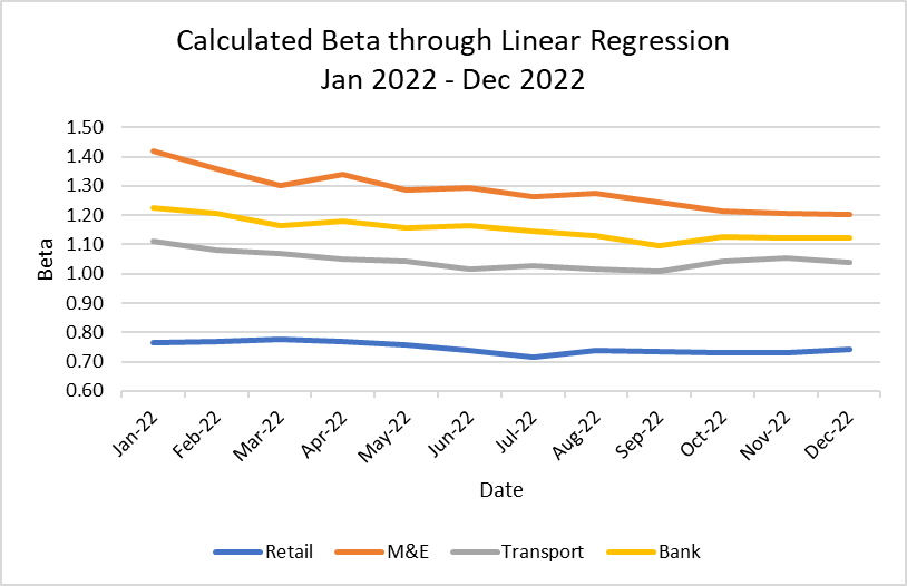
Figure 1: Calculated Beta through Linear Regression (2022)

5. Discussion

From the above regression results, we have the following findings:

1. The beta for each of the four industries is located in its specific interval without crossing over with that of other industries. As beta of a specific sector is a measure of the elasticity of its risk premium compared with that of the broad capital market, this result reflects the uniqueness of each sector’s performance during market turbulence.

2. Among the four sectors, media & entertainment exhibits the highest betas, followed by banks, transportations, and finally retail. Given our data timeline (Jan 2019 to Dec 2022) covers mainly the COVID-19 timeframe, the relative size of beta reflects the vulnerability level of the specific sector during the pandemic.

For example, the retail sector’s performance is closely linked to the consumption demand, which was deeply discouraged during the pandemic because of the restrictions on mobility. This in turn constrained the sector’s performance during the stock market rally in 2020 when the Fed was injecting liquidity through expansionary monetary policies since early 2020.

Similar observations can be found in the transportation sector, in which passenger traffic was severely disrupted during the pandemic, while partially offset by the surging financial performance of the marine shipping sector due to the capacity constraint in 2022.

As for media & entertainment, it was generally outperforming the market as people’s leisure activities were partially transferred to online entertainment during the pandemic. This in turn supports the strong growth of the monthly active users of the online entertainment platforms, as well as the traditional broadcasting sectors because people spent more time on consuming the contents.

Lastly, banks as the representative of the financial sector show moderate elasticity between M&E and transportation, indicating its relative neutrality among the four sectors.

3. All betas except that of the retail sector from Jan 2022 to Dec 2022 are generally moving down towards 1.0, meaning that the sector’s performance is steering towards that of the broad capital market. This observation is in tandem with the contradictory global financing condition last year that central banks globally including the Fed are raising the fund rates several times to control inflation.

The media & entertainment sector recorded the largest drop in beta from Jan 2022 to Dec 2022. This is possibly due to the global reopening after the spread out of the more infective yet less fatal XBB variant that made the governments to lift most mobility restrictions. As such the demand for digital contents post-pandemic is normalized to pre-pandemic level.

We also observed gradual termination of relief packages introduced by central banks during the pandemic. Since then, the banks were facing asset quality deterioration and provisioned more non-performing loans after the end of the loan moratorium. This negatively affected the bank’s financial performance. Having said that, the rate-hike environment is generally credit positive to the banking sector, as it should help improve the bank’s profitability, reflected from their larger net interest margin. This should partially offset the asset quality deterioration and make the beta of the sector still above 1.0 by the end of 2022.

The retail and transportation sector are less sensitive to the rate hike, as they were already discouraged by the mobility restrictions throughout the pandemic. The surging inflation since the early 2022 continued to erode the demand recovery and caused the severe backdrop of international trades in 2022, making the two sectors’ betas move in less degree over the year.

6. Conclusion

This research provides a rough estimation of the industry beta. However, there are several limitations within our research that prevent the result from guiding investment decision making. Firstly, the data set only covers three years of monthly data. This time series is less representative as the data are disrupted by an unprecedented pandemic during the last three years. The data frequency was also limited on a monthly basis to balance the efficiency and data accuracy. The results should be less optimal than that from data on a daily basis that has much more data points. Lastly, the CAPM model has too many assumptions which may not be suitable for real-world decision making. The model assumes the market is fully efficient and market participants are rational people, which may not be the case especially during the pandemic that investor sentiments are severely disrupted by panic and unprecedented monetary easing policies introduced by central banks.

Acknowledgements

Helena Xueqian Zhang and Qifeng Song contributed equally to this work and should be considered co-first authors.

References

[1]. W. Kenton, Capital asset pricing model (CAPM) and assumptions explained, in: Investopedia, 2023. Retrieved July 12, 2023, from https://www.investopedia.com/terms/c/capm.asp#:~:text=Despite%20its%20issues% 2C%20the%20CAPM,portfolio%20risk%20and%20expected%20return.
[2]. W. Kenton, Risk-free return calculations and examples, in: Investopedia, 2022. Retrieved July 12, 2023, from https://www.investopedia.com/terms/r/risk-freereturn.asp#:~:text=Risk%2Dfree%20return%20is%20the,a%20 specified%20period%20of%20time.
[3]. Investopedia, Why are T-Bills used when determining risk-free rates?, 2022. Retrieved July 12, 2023, from https://www.investopedia.com/ask/answers/040915/how-riskfree-rate-determined-when-calculating-market-risk-premium.asp#:~:text=The%20risk%2Dfree%20rate%20is,backed%20by%20the%20U.S.%20government.
[4]. Dan, Capital asset pricing model (CAPM), in: Strategic CFO, 2018. Retrieved July 12, 2023, from https://strategiccfo.com/articles/accounting/capital-asset-pricing-model-capm/.
[5]. A. Perković, Research of beta as adequate risk measure-is beta still alive?, in: Faculty of Economics Split Croatian Operational Research Review (CRORR), 2, 2011. DOI: https://hrcak.srce.hr/ 96623.
[6]. R. Elsas, M. El-Shaer, E. Theissen, Beta and returns revisited - Evidence from the German stock market, in: Journal of International Financial Markets, Institutions, and Money, 13(1), 2003, pp. 1-18. DOI: https://doi.org/10.1016/S1042-4431(02)00023-9.
[7]. C. Tofallis, Investment volatility: A critique of standard beta estimation and a simple way forward, in: European Journal of Operational Research, 187, 2011, pp. 1358-1367. DOI: https://doi.org/10.48550/arXiv.1109.4422.
[8]. E. Istanti, B. K. Negoro, Factors affecting stock beta in LQ-45 companies for the 2020-2021 period, in: International Journal of Economics and Management Research, 2(1), 2023. DOI: https://doi.org/10.55606/ijemr.v2i1.70.
[9]. V. J. Hooper, K. Ng, J. J. Reeves, Quarterly beta forecasting: An evaluation, in: International Journal of Forecasting, 24(3), 2008, pp. 480-489. DOI: https://doi.org/10.1016/j.ijforecast.2008.03.005.
[10]. J. Hong, X. Yu, W. Xiao, X. Zhang, The dispersion of beta estimates and the investors’ heterogeneous beliefs: Evidence from the stock market in China, in: International Review of Economics & Finance, 79, 2022, pp. 540-550. DOI: https://doi.org/10.1016/j.iref.2022.02.025.
[11]. R. Bradrania, J. F. Veron, W. Wu, The beta anomaly and the quality effect in international stock markets, in: Journal of Behavioral and Experimental Finance, 38, 2023. DOI: https://doi.org/10.1016/j.jbef.2023.100808.
[12]. S. M. Faisal, A. K. Khan, O. A. A. Aboud, Estimating beta (β) values of stocks in the creation of diversified portfolio - A detailed study, in: Applied Economics and Finance, 5(3), 2018. DOI: http://aef.redfame.com.
Cite this article
Zhang,H.;Song,Q. (2024). A Comparative Study of CAPM Based on the US Stock Market. Advances in Economics, Management and Political Sciences,82,64-71.
Data availability
The datasets used and/or analyzed during the current study will be available from the authors upon reasonable request.
Disclaimer/Publisher's Note
The statements, opinions and data contained in all publications are solely those of the individual author(s) and contributor(s) and not of EWA Publishing and/or the editor(s). EWA Publishing and/or the editor(s) disclaim responsibility for any injury to people or property resulting from any ideas, methods, instructions or products referred to in the content.
About volume
Volume title: Proceedings of the 2nd International Conference on Financial Technology and Business Analysis
© 2024 by the author(s). Licensee EWA Publishing, Oxford, UK. This article is an open access article distributed under the terms and
conditions of the Creative Commons Attribution (CC BY) license. Authors who
publish this series agree to the following terms:
1. Authors retain copyright and grant the series right of first publication with the work simultaneously licensed under a Creative Commons
Attribution License that allows others to share the work with an acknowledgment of the work's authorship and initial publication in this
series.
2. Authors are able to enter into separate, additional contractual arrangements for the non-exclusive distribution of the series's published
version of the work (e.g., post it to an institutional repository or publish it in a book), with an acknowledgment of its initial
publication in this series.
3. Authors are permitted and encouraged to post their work online (e.g., in institutional repositories or on their website) prior to and
during the submission process, as it can lead to productive exchanges, as well as earlier and greater citation of published work (See
Open access policy for details).