1. Introduction

1.1. Research Background and Significance

Time series modeling plays an important role in understanding and predicting trends in various fields, especially in economics and finance. By analyzing historical data, researchers and analysts can discover patterns, relationships, and trends that can provide valuable insights into future market movements, economic indicators, and financial results.

The focus of this study is to apply time series modeling techniques to NDX100 data, which stands for the NASDAQ 100 index. The NDX100 is an important benchmark for technology and growth companies, making it a popular choice for investors and analysts seeking investment opportunities in the sector.

By leveraging the historical price and volume data of the NDX100 index, the authoraim to develop robust time series models that can help us better understand the underlying dynamics of the market and make informed predictions about future movements. Through the use of statistical tools, econometric methods, and machine learning algorithms, the auhtor seek to uncover patterns, correlations, and trends that can guide decision-making in trading, investment, risk management, and policy formulation.

This study not only serves as a practical application of time series modeling in a real-world financial context but also demonstrates the importance of data-driven analysis in gaining a competitive edge in today's dynamic and fast-paced markets. By leveraging the power of historical data and advanced modeling techniques, investors can enhance their ability to predict market trends, reduce risks, and seize new opportunities in a constantly changing economic and financial market environment.

1.2. Literature Review

The NASDAQ 100 Index is an important indicator in the global financial market, including many high-tech companies. These companies are often leaders in technology, innovation and growth, making the index a key data for these industries. And as a representative of the technology industry, the NASDAQ 100 index has important reference value for investors and analysts. There has been great progress in the tech sector in recent years, and technology companies have continued to innovate, which has led to increased volatility in the Nasdaq 100 index. Therefore, the analysis and prediction of the NASDAQ 100 index has become particularly important.

Scientists use a variety of methods to analyze data from the Nasdaq 100 index. A common approach is to use an autoregressive integrated moving average model (ARIMA), which captures trends and cyclical changes in time series data [1]. In addition, machine learning algorithms are widely used in the prediction and analysis of the NASDAQ 100 index. For example, algorithms such as support vector machines (SVM) and Random Forest are used to build predictive models to help analyze market movements [2].

However, analysis of the Nasdaq 100 seems to have decreased in recent years. Despite the major breakthroughs made by technology companies in technology, the data analysis of the NASDAQ 100 index appears inadequate. Recently, there have been dramatic changes in the NASDAQ Index and increased market volatility, which makes the prediction and analysis of the NASDAQ 100 index particularly important [3].

This paper aims to use ARIMA model to analyze the NASDAQ 100 index data in the past three years, in order to fill the gap in the analysis of the index in recent years, and help better understand and predict the performance of the NASDAQ 100 index when the market fluctuations. Through in-depth analysis of the NASDAQ 100 index data, this paper can better grasp the pulse of the market and make more accurate investment decisions.

2. Methodology

2.1. Data Source and Processing

The data utilized in this paper was obtained from Investing(https://cn.investing.com/), a widely used financial data platform. The NDX100 index data covers the period from January 1, 2020, to December 31, 2023. The historical stock prices and related metrics were accessed through the Investing, with 1007 valid data.

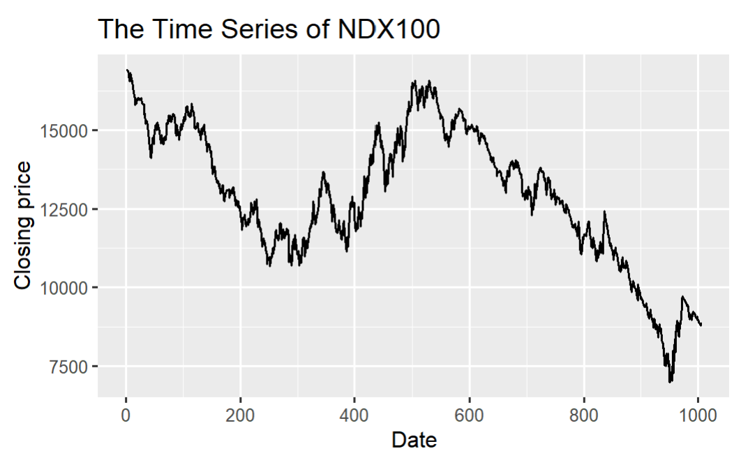
Figure 1: Time series of closing price of NDX100

From Figure 1, there is a clear trend in the NDX100 daily closing price index, and the market effectiveness hypothesis is based on the yield, so this paper transforms the daily closing price into the yield.

The return of the series is calculated by the change in the difference between the closing price of the index and the closing price of the current period:

\( {R_{t}}=\frac{{P_{t}}}{{P_{t-1}}} \) – 1 (1)

The author calculates the log return of the series in order to make the series stable and smooth:

\( {r_{t}}=ln\frac{{P_{t}}}{{P_{t-1}}}=ln⁡(1+{R_{t}}) \) (2)

2.2. ARIMA Model

The ARIMA model was established by Box George and JenkinsGwilym in 1970, and is also known as the Box-Jenkins method, in 1970. This method is widely regarded as one of the most important methods in financial forecasting. The ARIMA models have demonstrated a great ability to generate short-term predictions, consistently outperforming complex structural models in this regard [4].

3. Empirical Results Analysis

3.1. Autocorrelation Analysis

Autocorrelation analysis is a statistical method utilized to compare the similarity between a time series and itself after being lagged. In the context of analyzing the daily closing prices of the NDX100, autocorrelation becomes a valuable tool for understanding the temporal dependencies within the dataset. By calculating the correlation between the current day's closing price and its past values, autocorrelation helps identify patterns, trends, or cycles in the stock market.

In the autocorrelation test, the study aims to analyze whether the NDX100 data exhibits random distribution. The results of the autocorrelation test are shown in Figures 2-3.If the data lacks autocorrelation, it suggests randomness, implying that future developments are independent of past performance. Consequently, a low autocorrelation in the series aligns with the hypothesis that the market adheres to weak form efficiency.

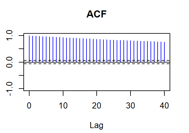
Figure 2: ACF plot of NDX100 data

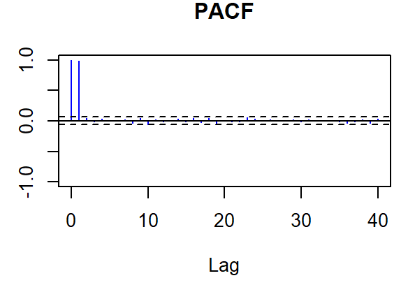
Figure 3: PACF plot of NDX100 data

White noise is a concept in time series analysis where the data points are independent and evenly distributed the mean is zero and the variance is constant. To check whether a dataset is white noise, people can use statistical tests such as Ljung-Box tests or check the autocorrelation function. The author tests the NDX100 data using functions such as Box.test() (Ljung-Box test) to analyze the autocorrelation properties of the dataset. If the autocorrelation is close to zero and falls within the confidence band, the data can be treated as white noise. The results are shown in Table1:

Table 1: The test results of Ljung-Box test

The residual sequence diagram of NDX100 data is shown in Figure 4.

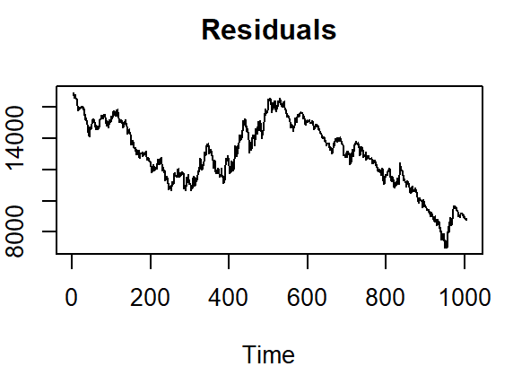
Figure 4: Residuals of NDX100 data

This article uses Q-Q diagram to test the normal distribution of the sequence, which are shown in Figure 5. From Figure5, it shows that the sequence may not conform to the normal distribution at this time.

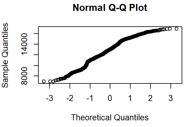
Figure 5: Q-Q plot of NDX100 data

The p-value result from table 1 suggests the rejection of the null hypothesis that the residuals are independent and identically distributed noise. Here's a brief interpretation of the key test statistics:

Upon observation, the p-value from the Ljung-Box test is less than 0.05. It leads to the rejection of the null hypothesis, indicating that the series is not white noise. Non-white noise implies a lack of pure-random distribution, leading to a tentative conclusion that the domestic market does not align with the hypothesis of a weak efficiency market. Observation of the Augmented Dickey-Fuller (ADF) test plot reveals a significant short-term autocorrelation in the first period, which is further evidence that the data is not a white noise series.

In summary, all the test statistics strongly reject the hypothesis of independent and identically distributed residuals, implying the presence of autocorrelation or systematic patterns in the residuals of NDX100 data.

3.2. ADF Test

The Augmented Dickey-Fuller (ADF) test is employed to formally evaluate the presence of a unit root. The ADF test results are shown in table 2.

Table 2: ADF test result

The ADF test statistic is -1.5733, surpassing the critical values for significance. The p-value indicates a rejection of the null hypothesis, suggesting evidence against the presence of a unit root. The time series appears to be stationary after differencing.

3.3. ARIMA Model

A nonseasonal ARIMA model, classified as ARIMA (p, d, q), where: p is Autoregressive (AR) coefficient, d is after how many differences, data reaches its stationary, q is Moving Average (MA) coefficient

Applying differencing (diff()) to the original time series is employed to assess the effectiveness of removing trends and achieving stationary. The sequence after differentiation is shown in Figure 6.

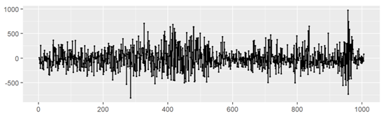
Figure 6: Plot after 1st-oder differencing

As Figure 6 shown, the data is stationary out after the first-order differencing. So let d = 1.

The next step is to select best p and q in the ARIMA model. In order to find suitable p and q, this paper utilized the ACF plot and PACF plot to determine q and p respectively.

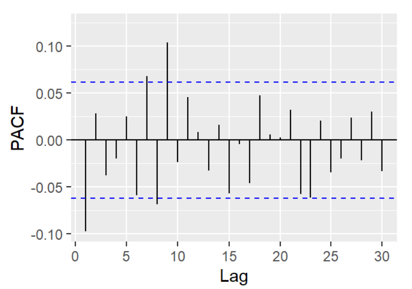
Figure 7: PACF plot after 1st-oder differencing

Significant spikes outside the blue boundary of the PACF plot give the order of the AR model. By observation, there are 4 significant spikes outside critical value range. So, p = 4. The MA( q) model calculates its forecasts by taking a weighted average of past errors. It captures trends and patterns in time series data. If the plot has a sharp cutoff after the lag, q can be determined from the ACF plot.

Similar to the selection of the AR model p, in order q to select the appropriate order for the MA model, the author need to analyze all spikes above the blue region.

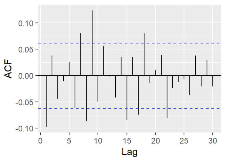
Figure 8: ACF plot after 1st-order differencing

From the above plot, it shows that there are sharp cutoffs after lag1, lag7, lag8, lag9, lag15, lag18 and lag22. Let q = 1, 7, 8, 9, 15, 18, or 22. A better ARIMA model can be chose by comparing AIC and BIC value.

AIC and BIC are two criteria that measure the goodness of fit of a statistical model, considering both the complexity and the accuracy of the model, which quantifies how well the model fits the data, and penalize the model for having more parameters, which increases the risk of over fitting. A lower AIC or BIC value indicates a better model.

\( AIC = 2K – 2ln(L) \) (3)

Where: K: The number of independent variables, ln(L): The log-likelihood estimate [5].

\( BIC=Kln(n)-2ln(L) \) (4)

where n is sample size [6-8].

By applying function BIC(), the BIC values are shown in Table3:

Table 3: The test results of Ljung-Box test

By comparing the value in the Table3, it is obvious that ARIMA (4,1,1) has the smallest AIC and BIC value, which imply ARIMA (4,1,1) is the best fit.

ARIMA is a very powerful time series prediction model, but the process of data preparation and parameter adjustment is very time-consuming [9,10]. Auto ARIMA makes the whole task very simple, eliminating the process of sequence stabilization, determining d values, creating ACF values and PACF graphs, determining p values and q values

Use function auto.arima, the results gives that ARIMA (4,1,1) is the best fit. In this part, ARIMA(4,1,1) model is chosen for prediction and conduct Ljung-Box test, the estimate results are shown in Table 4.

Table 4: ARIMA (4,1,1) with drift

From the results in Table 4, it shows that the ARIMA model has a good fitting effect on the model. At the same time, the residual plot of the resulting model further reveals that the model has stability and can be used for data fitting (see Figure 9).

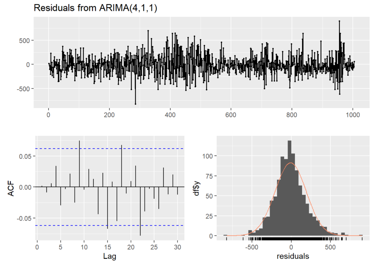
Figure 9: Residuals from ARIMA (4,1,1)

4. Conclusion

The unit root analysis, particularly the ADF test, sheds light on the stationary of the "profit" time series. With a p-value of 0.03321 indicating stationary after differencing, it suggests that the profit data exhibits stable, predictable patterns over time. Given this finding, it's prudent to consider the implications for refining the chosen ARIMA (4,1,1) model. While the ARIMA model captures the autocorrelation and seasonality in the data, it may warrant further evaluation and refinement to enhance forecasting accuracy and analytical insights. The ARIMA(4,1,1) model with drift reveals significant coefficients, particularly a negative correlation in returns between the last two periods and the current period. This suggests a potential pattern of negative momentum in the profit series, influencing trading decisions and market efficiency considerations. Additionally, the non-significant autocorrelation in the residuals supports the model's adequacy in capturing temporal dynamics, further validating its utility in forecasting and analysis of the profit time series.

Future research could focus on further refining the ARIMA model by considering additional external variables or alternative specifications. This could improve forecasting accuracy and have a better understanding of the dynamics in financial market. The insights and methodologies presented in the paper can be applied to other financial time series datasets, providing valuable guidance for analysts and researchers in forecasting and analyzing market trends. In the meanwhile, the findings of the paper could have implications for policymakers and market participants, highlighting the importance of considering momentum effects in trading strategies and market efficiency considerations.

References

[1]. G. Peter. Zhang. (2003). Time series forecasting using a hybrid ARIMA and neural network model, Neurocomputing.
[2]. Madge, S., & Bhatt, S. (2015). Predicting stock price direction using support vector machines. Independent work report spring, 45.
[3]. Nicholas Megaw, George Steer. (2023). Nasdaq records best quarter since 2020 after volatile start to year, Financial Times, Retrieved from https://www.ft.com/content/01af6fd2-5456-4d9c-894f-dd80235308fd.
[4]. Box, George; Jenkins, Gwilym (1970). Time Series Analysis: Forecasting and Control. San Francisco: Holden-Day.
[5]. H. Akaike. (1974). A new look at the statistical model identification, IEEE Transactions on Automatic Control, 19(6): 716-723.
[6]. Schwarz, Gideon E. (1978). Estimating the dimension of a model, Annals of Statistics, 6 (2): 461–464.
[7]. Benvenuto, D., Giovanetti, M., Vassallo, L., Angeletti, S., & Ciccozzi, M. (2020). Application of the ARIMA model on the COVID-2019 epidemic dataset. Data in brief, 29, 105340.
[8]. Ho, S. L. et al. (1998). The use of ARIMA models for reliability forecasting and analysis. Computers & industrial engineering, 35(1-2), 213-216.
[9]. Fattah, J., Ezzine, L., Aman, Z., El Moussami, H., & Lachhab, A. (2018). Forecasting of demand using ARIMA model. International Journal of Engineering Business Management, 10, 1847979018808673.
[10]. Chodakowska, E., Nazarko, J., Nazarko, Ł., Rabayah, H. S., Abendeh, R. M., & Alawneh, R. (2023). Arima models in solar radiation forecasting in different geographic locations. Energies, 16(13), 5029.
Cite this article
Yi,Z. (2024). Analysis of Stock Market Prices Based on ARIMA Model: Evidence from NASDAQ 100 Index. Advances in Economics, Management and Political Sciences,88,89-98.
Data availability
The datasets used and/or analyzed during the current study will be available from the authors upon reasonable request.
Disclaimer/Publisher's Note
The statements, opinions and data contained in all publications are solely those of the individual author(s) and contributor(s) and not of EWA Publishing and/or the editor(s). EWA Publishing and/or the editor(s) disclaim responsibility for any injury to people or property resulting from any ideas, methods, instructions or products referred to in the content.
About volume
Volume title: Proceedings of the 2nd International Conference on Management Research and Economic Development
© 2024 by the author(s). Licensee EWA Publishing, Oxford, UK. This article is an open access article distributed under the terms and
conditions of the Creative Commons Attribution (CC BY) license. Authors who
publish this series agree to the following terms:
1. Authors retain copyright and grant the series right of first publication with the work simultaneously licensed under a Creative Commons
Attribution License that allows others to share the work with an acknowledgment of the work's authorship and initial publication in this
series.
2. Authors are able to enter into separate, additional contractual arrangements for the non-exclusive distribution of the series's published
version of the work (e.g., post it to an institutional repository or publish it in a book), with an acknowledgment of its initial
publication in this series.
3. Authors are permitted and encouraged to post their work online (e.g., in institutional repositories or on their website) prior to and
during the submission process, as it can lead to productive exchanges, as well as earlier and greater citation of published work (See
Open access policy for details).