1. Introduction

Known as the biggest and most extensive market mechanisms in the world, the carbon trading market has played a crucial role in reducing carbon emissions worldwide. As the carbon market has matured, derivative markets, including those for carbon futures, options, and forwards, have become increasingly active. The volatility of carbon quota pricing has noticeably increased in tandem with this expansion. The price of carbon futures has fluctuated significantly over the past few decades, according to statistics from the Intercontinental Exchange (ICE). These price swings are important because they influence how market players behave. However, price discrepancies may contribute to market inefficiencies, causing deviations from the true supply-demand equilibrium and undermining the market's effectiveness.

The financialization of commodity futures has led to increased price volatility and greater market uncertainty, signalling higher systemic risks due to the heightened co-movements in futures prices [1]. For instance, EU Allowance (EUA) prices, which remained below 10 euros until the ETS's fourth phase reform in 2018, saw a slight decline in 2019 due to the COVID-19 pandemic, reflecting market expectations of reduced economic activities and global energy demand. It is noteworthy that crude oil and natural gas futures have exhibited heightened sensitivity and more frequent volatility. In 2021, the demand for natural gas saw a marked increase due to the economic rebound following the pandemic and the growing preference for coal as an alternative energy source, even though it emits more CO2. This shift contributed to substantial rises in the prices of EUAs, setting new record levels. However, the data currently accessible does not clearly show a correlation between these markets. Previous studies indicate that futures returns and volatility share long-term cointegration relationships [2], prompting the use of the Dynamic Conditional Correlation Generalized Autoregressive Conditional Heteroskedasticity model (DCC-GARCH) in this study to further investigate these dynamics.

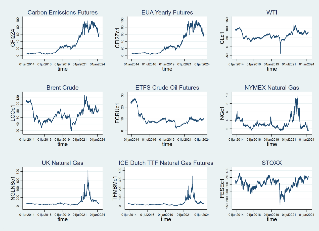
Figure 1: daily closing price trends of 9 futures between November 21,2013 and March 28, 2024.

Carbon emission futures have recently become prominent financial instruments, yet there hasn't been much research done on the dynamic relationships between future energy and carbon emission trends. By investigating the interactions between these markets within the framework of changing international environmental regulations, this study seeks to close this gap. This study provides valuable insights for investors, governments, and businesses through its analysis of dynamic correlations between carbon emission futures and energy futures, also illuminating potential impacts of carbon costs on energy market prices.

This paper contributes to the existing literature by analysing the dynamic correlations over extended periods and examining the characteristics and variations in these correlations. Additionally, it evaluates the short- and long-term impacts of various marketplaces and compares dynamic conditional correlation coefficients across various markets and locations. This research serves as a basis for future policy-making and facilitates the assessment of the effects of different environmental policies on the energy market.

The paper is organized as follows: Section 2 offers a review of relevant literature; Section 3 describes the data and methodologies used to compute dynamic correlations using the DCC-GARCH model; Section 4 presents the empirical findings of the study, while Section 5 provides conclusions and policy recommendations.

2. Literature Review

Numerous studies have investigated dynamic correlations in futures markets across various asset, including commodities, currencies, and equities. Comprehending the dynamic correlations among distinct futures markets is crucial for effective risk mitigation, portfolio diversification, and trading tactics. The financialization of energy markets promotes changes in energy price volatility and increases liquidity between energy markets [3]. The pattern and intensity of volatility fluctuations over the period vary across different futures markets, implying that varying levels of sensitivity to economic changes further affect the strength of these correlations [4]. Despite financial uncertainty significantly impacting crude oil futures trends negatively, WTI and Brent crude oil still exhibit strong correlations and mutual influence [5]. There exists a bidirectional asymmetrical relationship between crude oil markets and agricultural commodity markets, exacerbated during financial crises, the COVID-19 pandemic, and oil market crashes [6-7]. COVID-19 has had significant and enduring impacts on the risk interdependence between energy, agriculture, and other commodities [8].

Methodologically, scholars employ various approaches to analysis the data, such as Vector Autoregressive (VAR) models, cointegration analysis, Multivariate GARCH models, DCC-GARCH models, and the Diebold and Yilmaz (DY) method [9-13]. Henriques and Sadorsky were among the early adopters of VAR models to study the impact of oil prices on stock markets [14]. Bondia et al. utilized cointegration models and discovered significant short-term relationships between alternative energy stock prices and oil prices, though these relationships were not significant in the long term [15]. Zhang et al. using the DCC-GARCH dynamic connectivity approach, analysed the dynamic connectivity between ESG stock indices and carbon emission futures, finding carbon emission futures to be transmitters of volatility while green bonds act as receivers [16]. Sadorsky compared four different multivariate GARCH models (BEKK, Diagonal, Constant Conditional Correlation, and Dynamic Conditional Correlation) and found the dynamic conditional correlation model most suitable for analyzing time series data such as stock prices [17]. With fixed correlation coefficients, the hedging ratio calculated using the DCC-GARCH model proves to be more precise than the one derived from the GARCH model [18].

The carbon financial market is highly volatile, unpredictable, and impacted by a number of variables, including politics, the economy, and commodities prices. Carbon emission quotas and energy markets demonstrate significant interdependence, with European Union emission quotas and futures markets showing close volatility relationships [19]. According to a report from the China International Capital Corporation Limited (CICC) Global Institute, futures market trading volume accounted for 90% of the total carbon quota trading volume during the second phase of the EU carbon market construction. The coal market exhibits significant one-way spillover effects on the carbon market, while the carbon market, in turn, has substantial spillover effects on the natural gas market. Over time, the carbon market and fossil energy markets demonstrate strong positive correlations [20]. When the economy is strong and carbon prices are high, natural gas prices having less impact on carbon prices compared to oil and coal prices [21]. Over the long term, uncertainty in economic policies substantially reduces returns on carbon futures prices. The COVID-19 pandemic impacts their short- to medium-term performance by affecting the spillover and correlation between Economic Policy Uncertainty (EPU) and the returns on carbon futures prices [22]. Due to the immaturity of the EU carbon trading system, inefficient trading, and the game of carbon emission rights allocation based on national welfare interests between countries and blocs, the complexity of EUA futures is observed [23].

Previous research has highlighted the time-varying character of correlations and the importance of employing appropriate methodologies to analyze them. By utilizing advanced econometric techniques, researchers can gain further insights into the dynamic correlations between futures contracts, contributing to improved risk management and investment strategies in financial markets. Whether in energy futures markets or carbon markets, both of which are highly susceptible to external influences. However, there is limited literature utilizing the DCC-GARCH method to analyze the correlation of futures over longer time intervals. Hence, to assess if the correlation between carbon futures and energy futures persists over a longer duration, this study builds upon previous research by broadening the timeframe of the data analyzed.

3. Data and Methodology

3.1. Variables and Data

Analyzing the dynamic correlation between energy and carbon futures is the goal of this research. To achieve this, EUA futures traded at the Intercontinental Exchange (ICE) and the European Energy Exchange (EEX) were selected. Previous research has demonstrated that changes in coal, crude oil, and natural gas prices significantly affect short-term emission quota prices in the United States Emissions Trading System (ETS) [24-25]. Therefore, we choose the prices of Crude Oil (WTI, Brent, ETFS), Natural Gas (NYMEX Natural Gas, UK Natural Gas, ICE Dutch TTF Natural Gas), and European STOXX Oil & Gas futures. The sample period for this dataset spans from 21 November 2013 to 28 March 2024, and all this data can be obtained from Investing.com.

Considering the different units of futures prices in each contract, we use the returns of the futures \( {(rf_{t}}) \) for dynamic correlation analysis. The futures prices are expressed in \( {P_{t}} \) separately and the daily returns are computed as follows:

\( {rf_{t}}=ln{(\frac{{P_{t}}}{{P_{t-1}}})} \) (1)

Table 1 displays the descriptive statistics for the daily returns. Across the seven sequences of returns, the mean is approximately zero, indicating proximity to zero average returns. The wide gap between the highest and lowest values for most variables indicates potential outliers or extreme values in these futures returns.

Table 1: Descriptive statistics for the daily returns of futures.

The data distribution exhibits left skewness with higher kurtosis values, indicating a highly concentrated distribution with sharp peaks and one or more extreme tail values. Furthermore, Jarque-Bera test statistics reveal outcomes that do not align with a normal distribution across extended periods, suggesting a non-linear process. Time series modeling is underpinned by the stationarity of each return series, as evidenced by the Augmented Dickey-Fuller (ADF) unit root test results.

3.2. DCC-GARCH Model

In finance, time series data often exhibit autocorrelation. Initially, scholars typically assumed constant variance in their research. However, in practical applications, time series may display volatility clustering. Thus, Engle proposed using Autoregressive Conditional Heteroskedasticity (ARCH) to assess variance fluctuations. Building on this, Bollerslev introduced a variance autoregressive component, thereby enhancing practicality of this model [26-27]. Leveraging Bollerslev's constant conditional correlation estimator, Engle further introduced Dynamic Conditional Correlation (DCC) estimators. Without the complexity of conventional multivariate GARCH, this technique provides the flexibility of univariate GARCH [28]. The DCC-GARCH model calculates dynamic interconnections helps avoid the loss of observational data, thereby highlighting its reliability and benefits compared to unconditional correlation analysis. The model accounts for heteroskedasticity by estimating the correlation of standardized residuals, which reduces volatility biases in DCC analyses [29]. The DCC-GARCH model is computed through a two-stage process: initially, a univariate GARCH model is estimated for each sequence of residuals; subsequently, the residuals, adjusted by the standard deviation calculated in the first stage, are utilized to estimate parameters for dynamic correlation.

According to Engle, assume that \( {E_{t-1}}[{ε_{t}}]=0 \) for \( t=1,⋯,n \) and \( {E_{t-1}}[{ε_{t}}{ε_{t}} \prime ]={H_{t}} \) are satisfied, where \( {E_{t}}[ \cdot ] \) is the conditional expectation. The model can be specified as follows:

\( {H_{t}}={D_{t}}{R_{t}}{D_{t}} \) (2)

\( {{[R_{t}}]_{i,j}}=\frac{{q_{i,j,t}}}{\sqrt[]{{q_{i,i,t}}{q_{j,j,t}}}} \) (3)

\( {q_{i,j,t}}=(1-λ)({ε_{i,t-1}}{ε_{j,t-1}})+λ({q_{i,j,t-1}}) \) (4)

\( {Q_{t}}=(1-α-β)\bar{Q}+α({ε_{t-1}}ε_{t-1}^{ \prime })+β{Q_{t-1}} \) (5)

Where \( {H_{t}} \) represents the conditional covariance matrix, \( {R_{t}} \) denotes the conditional correlation matrix, and \( {D_{t}} \) is a diagonal matrix containing the time-varying standard deviations of the conditional variance \( \sqrt[]{{h_{i,t}}} \) derived from the GARCH model, \( \bar{Q} \) represents the time-varying unconditional correlation matrix of the standardized residuals \( ε \) , and \( 0 \lt α+β \lt 1 \) . Due to space limit, a detailed description of the DCC-GARCH model can be found in Engle (2002).

The dynamic correlation coefficient \( α \) represents the short-term persistence of dynamic correlations by demonstrating the impact of the standardized residuals from the previous period on the dynamic correlation coefficients. In contrast, the dynamic correlation coefficient \( β \) represents the long-term persistence of the correlation between assets, indicating the effect of the prior period's correlation coefficients on the current period. The larger the combined value of \( α \) and \( β \) , the more persistent the correlation.

We first estimate the bivariate Vector Autoregressive model (VAR), as indicated:

\( \begin{cases} \begin{array}{c} {rf_{1,t}}={μ_{1}}+\sum _{i=1}^{n}{a_{1,i}}{rf_{1,t-1}}+\sum _{i=1}^{n}{b_{1,i}}{rf_{2,t-1}}+{ε_{1,t}} \\ {rf_{2,t}}={μ_{2}}+\sum _{i=1}^{n}{a_{2,i}}{rf_{1,t-1}}+\sum _{i=1}^{n}{b_{2,i}}{rf_{2,t-1}}+{ε_{2,t}} \end{array} \end{cases} \) (6)

Then we estimate the DCC (1,1) model using the VAR residuals, which is defined as:

\( {h_{it}}={γ_{t}}+{α_{i,t}}rf_{i,t-1}^{2}+{β_{i,t}}{h_{i,t-1}} \) (7)

\( {Q_{t}}=(1-{α_{1}}-{β_{1}})\bar{Q}+{α_{1}}({ε_{t-1}}ε_{t-1}^{ \prime })+{β_{1}}{Q_{t-1}} \) (8)

4. Empirical Results

4.1. The Dynamic Conditional Correlations

The Pearson correlation test offers correlation coefficients between -1 and 1, values close to -1 indicate stronger negative correlations, those near 1 indicate stronger positive, and values around 0 suggest weak or non-existent relationships. The correlation matrix derived from Pearson correlation tests displays the relationships between variables, as shown in Table 2. A very strong positive correlation between the prices of carbon futures in the two markets is indicated by the correlation coefficient of 0.996 between the variables cfi2zc1 and cfi2z4, for example, suggesting limited prospects for arbitrage between them. Although the correlation between energy and carbon futures is not as strong, it is still pretty similar.

Table 2: Pearson correlation coefficient between daily returns.

Time-varying conditional correlation exists between energy and carbon futures. The majority of the DCC coefficients relating energy market returns to carbon are positive, except for a few exceptional negative values, as shown in Figure 2, suggesting a certain amount of synergy between the carbon and energy futures markets. The conditional correlation coefficients between crude oil futures and the carbon futures show more dramatic fluctuations than those for natural gas futures, but they generally remain positive throughout most trading periods. After the second quarter of 2019, oil prices fell continuously due to factors such as intensified international trade disputes and weak oil demand. In the first quarter of 2022, international oil prices rose influenced by the Russia-Ukraine conflict. Nevertheless, the carbon market exhibited no immediate short-term impact, resulting in a notable decrease in the DCC coefficients during these periods, which suggests a reduction in the risk synergy effect between the two markets. Periods of negative correlation imply opportunities for portfolio diversification, and investment decisions during these periods should also consider various products. The synergy effect in the natural gas market is likewise impacted by events like the conflict between Russia and Ukraine; however, unlike the crude oil futures, the dynamic conditional correlation between the carbon futures and natural gas futures shows only a slight tendency to vary over time. This implies that managers of the carbon market ought to be more aware of changes in the price of crude oil.

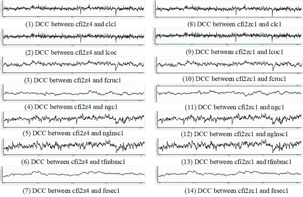
Figure 2: Dynamic conditional correlation (DCC) between carbon futures and energy futures markets.

4.2. DCC‐GARCH Results

The estimated results of the DCC-GARCH model between carbon and energy futures are presented in Table 3. Energy and carbon futures both show persistence in long-term impacts and short-term market adjustments. The \( α+β \) for the combinations of energy and carbon futures are close to, but less than 1, indicating a mean-reverting return process with significant volatility clustering present in each pair. This suggests that rising prices of energy and carbon futures consistently have a volatile effect on future pricing. The relationship between the natural gas futures and the carbon futures shows greater persistence compared to that between crude oil futures and carbon futures, as evidenced by a higher sum of \( α+β \) for the former. The \( α+β \) for WTI crude oil and Brent crude oil compared to ETFS Crude Oil is smaller, suggesting a stronger and longer-lasting relationship between the carbon futures and European crude oil futures. With increasing short-term persistency of dynamic conditional correlation influences on the returns of the crude oil and carbon markets, the \( α \) coefficient for each pair is significant, suggesting short-term predictability in the fluctuations of correlation between the energy and carbon markets. The \( β \) for each pair is significant, demonstrating the substantial long-term persistence effects between the carbon and energy futures markets. The \( β \) value for the combination of natural gas market is significantly close to 1, indicating that the long-term persistency of price movement impacts is crucial for all long-term forecasts of DCC coefficients in all scenarios.

Table 3: The estimated results of the DCC-GARCH model between futures.

Note: Robust standard errors in parentheses. ***, ** and * indicate the significance level at 1%, 5%, 10% respectively.

5. Conclusions

This paper explores the dynamic conditional correlation of energy futures and carbon futures. The findings show that: Firstly, the same type of carbon futures traded in different regional futures markets exhibit extremely strong correlations, with limited arbitrage opportunities between markets. Secondly, a noteworthy positive conditional correlation exists between the carbon futures and energy futures markets, indicating a certain level of risk synergy effect. However, this tends to change over time, with the crude oil market combination showing more significant fluctuations in conditional correlation. Thirdly, both the energy and carbon futures markets exhibit notable long-term persistence effects along with short-term predictability, with stronger persistency observed in the natural gas futures combination.

Building on research that explores the connection between energy and carbon markets, this study provides more comprehensive data for market analysis and forecasting. Carbon market investors can refer to the changing trends in market correlations, incorporate natural gas futures and other varieties, and construct effective investment portfolios to mitigate extreme risks. Market regulators can better predict the intensity of extreme risks on market impact and their effects on dynamic conditional correlations between markets, taking timely measures to maintain market stability and reduce the impact of arbitrage activities. Governments should make more concerted efforts to transition to low-carbon energy, reduce dependence on fossil fuels, and build long-term robust investment portfolios to lessen the effects of changes in the prices of crude oil futures brought on by outside market shocks.

References

[1]. Zhang, D., Broadstock, D.C. Global financial crisis and rising connectedness in the international commodity markets. International review of financial analysis. 68,101239 (2018). https://doi.org/10.1016/j.irfa.2018.08.003
[2]. Yang, J., Zhou, Y. Return and volatility transmission between China’s and international crude oil futures markets: a first look. The Journal of Futures Markets. 40 (6), 860–884 (2020). https://doi.org/10.1002/fut.22103
[3]. Fattouh, B., Kilian, L., Mahadeva, L. (2013). The role of speculation in oil markets: what have we learned so far? The Energy Journal, 34, 7–33. https://doi.org/10.5547/01956574.34.3.2
[4]. Kuruppuarachchi, D., Premachandra, I.M. (2016). Information spillover dynamics of the energy futures market sector: A novel common factor approach. Energy Economics, 57, 277-294. https://doi.org/10.1016/j.eneco.2016.05.015
[5]. Liu, M., Lee, C. (2021). Capturing the dynamics of the China crude oil futures: Markov switching, co-movement, and volatility forecasting. Energy Economics, 103, 105622. https://doi.org/10.1016/j.eneco.2021.105622
[6]. Dahl, R. E., Oglend, A., & Yahya, M. (2020). Dynamics of volatility spillover in commodity markets: Linking crude oil to agriculture. Journal of Commodity Markets, 20, 100111. https://doi.org/10.1016/j.jcomm.2019.100111
[7]. Chen, Z., Yan, B., Kang, H. (2022). Dynamic correlation between crude oil and agricultural futures markets. Review of Development Economics, 26, 1798–1849. https://doi.org/10.1111/rode.12885
[8]. Qiao, T., Han, L. (2023). COVID-19 and tail risk contagion across commodity futures markets. The Journal of Futures Markets, 43, 242–272. https://doi.org/10.1002/fut.22388
[9]. Sims, C.A. (1980). Macroeconomics and Reality. Econometrica: Journal of the Econometric Society, 48, 1-48. https://doi.org/10.2307/1912017
[10]. Gonzalo, J., & Granger, C. (1995). Estimation of Common Long-Memory Components in Cointegrated Systems. Journal of Business & Economic Statistics, 13(1), 27–35. https://doi.org/10.1080/07350015.1995.10524576
[11]. Tse, Y. K., & Tsui, A. K. C. (2002). A Multivariate Generalized Autoregressive Conditional Heteroscedasticity Model With Time-Varying Correlations. Journal of Business & Economic Statistics, 20(3), 351–362. https://doi.org/10.1198/073500102288618496
[12]. Engle, R. (2002). Dynamic Conditional Correlation: A Simple Class of Multivariate Generalized Autoregressive Conditional Heteroskedasticity Models. Journal of Business & Economic Statistics, 20(3), 339–350. https://doi.org/10.1198/073500102288618487
[13]. Diebold, F.X. and Yilmaz, K. (2009), Measuring Financial Asset Return and Volatility Spillovers, with Application to Global Equity Markets. The Economic Journal, 119: 158-171. https://doi.org/10.1111/j.1468-0297.2008.02208.x
[14]. Henriques, I. and Sadorsky, P. (2008). Oil prices and the stock prices of alternative energy companies. Energy Economics, 30 (3), 998-1010. https://doi.org/10.1016/J.ENECO.2007.11.001
[15]. Bondia, R., Ghosh, S., Kanjilal, K. (2016). International crude oil prices and the stock prices of clean energy and technology companies: Evidence from non-linear cointegration tests with unknown structural breaks. Energy, 101, 558-565. https://doi.org/10.1016/j.energy.2016.02.031
[16]. Zhang, W., He, X., Hamori, S. (2022). Volatility spillover and investment strategies among sustainability-related financial indexes: Evidence from the DCC-GARCH-based dynamic connectedness and DCC-GARCH t-copula approach. International Review of Financial Analysis, 83, 102223. https://doi.org/10.1016/j.irfa.2022.102223
[17]. Sadorsky, P. (2012). Correlations and volatility spillovers between oil prices and the stock prices of clean energy and technology companies. Energy Economics, 34(1), 248-255. https://doi.org/10.1016/j.eneco.2011.03.006
[18]. Zhou, J. (2016). Hedging performance of REIT index futures: A comparison of alternative hedge ratio estimation methods. Economic modelling, 52, 690-698. https://doi.org/10.1016/j.econmod.2015.10.009
[19]. Ritter D. (2012). Price discovery and volatility spillovers in the European Union emissions trading scheme: a high-frequency analysis. Journal of Banking & Finance, 36(3), 774-785. https://doi.org/10.1016/j.jbankfin.2011.09.009
[20]. Zhang, Y. and Sun, Y. (2016). The dynamic volatility spillover between European carbon trading market and fossil energy market. Journal of Cleaner Production, 112(4), 2654-2663. https://doi.org/10.1016/j.jclepro.2015.09.118
[21]. Duan, K., Ren, X., Shi, Y., Mishra, T., & Yan, C. (2021). The marginal impacts of energy prices on carbon price variations: Evidence from a quantile-on-quantile approach. Energy Economics, 95, 105131. https://doi.org/10.1016/j.eneco.2021.105131
[22]. Dou, Y., Li, Y., Dong, K., Ren, X. (2021). Dynamic linkages between economic policy uncertainty and the carbon futures market: Does Covid-19 pandemic matter? Resources Policy, 75, 102455. https://doi.org/10.1016/j.resourpol.2021.102455
[23]. Chen, J., Ma, S., Wu, Y. (2021). International carbon financial market prediction using particle swarm optimization and support vector machine. Journal of Ambient Intelligence and Humanized Computing, 13,5699 - 5713. https://doi.org/10.1007/s12652-021-03240-7
[24]. Kim, H.S. and Koo, W.W. (2010). Factors affecting the carbon allowance market in the US. Energy Policy, 38(4), 1879-1884. https://doi.org/10.1016/j.enpol.2009.11.066
[25]. Zhu, B., Ye, S., Han, D., Wang, P., He, K., Wei, Y., Xie, R. (2019). A multiscale analysis for carbon price drivers. Energy Economics, 78, 202-216. https://doi.org/10.1016/j.eneco.2018.11.007
[26]. Engle, R.F. (1982). Autoregressive conditional heteroscedasticity with estimates of the variance of United Kingdom inflation. Econometrica, 50, 987-1007. https://doi.org/10.2307/1912773
[27]. Bollerslev, T. (1986). Generalized autoregressive conditional heteroskedasticity. Journal of Econometrics, 31(3), 307-327. https://doi.org/10.1016/0304-4076(86)90063-1
[28]. Bollerslev, T. (1990). Modeling the Coherence in Short-run Nominal Exchange Rates: A Multivariate Generalized ARCH Model. Review of Economics and Statistics, 72,498-505. https://doi.org/10.2307/2109358
[29]. Gabauer, D. (2020). Volatility impulse response analysis for DCC-GARCH models: the role of volatility transmission mechanisms. Journal of Forecasting. 39, 788–796. https://doi.org/ 10.1002/for.2648
Cite this article
Liu,S. (2024). Dynamic Correlations Between Carbon Futures and Energy Futures Markets. Advances in Economics, Management and Political Sciences,91,120-129.
Data availability
The datasets used and/or analyzed during the current study will be available from the authors upon reasonable request.
Disclaimer/Publisher's Note
The statements, opinions and data contained in all publications are solely those of the individual author(s) and contributor(s) and not of EWA Publishing and/or the editor(s). EWA Publishing and/or the editor(s) disclaim responsibility for any injury to people or property resulting from any ideas, methods, instructions or products referred to in the content.
About volume
Volume title: Proceedings of the 2nd International Conference on Management Research and Economic Development
© 2024 by the author(s). Licensee EWA Publishing, Oxford, UK. This article is an open access article distributed under the terms and
conditions of the Creative Commons Attribution (CC BY) license. Authors who
publish this series agree to the following terms:
1. Authors retain copyright and grant the series right of first publication with the work simultaneously licensed under a Creative Commons
Attribution License that allows others to share the work with an acknowledgment of the work's authorship and initial publication in this
series.
2. Authors are able to enter into separate, additional contractual arrangements for the non-exclusive distribution of the series's published
version of the work (e.g., post it to an institutional repository or publish it in a book), with an acknowledgment of its initial
publication in this series.
3. Authors are permitted and encouraged to post their work online (e.g., in institutional repositories or on their website) prior to and
during the submission process, as it can lead to productive exchanges, as well as earlier and greater citation of published work (See
Open access policy for details).