1. Introduction

As an alternate type of digital currency that functions differently from conventional financial institutions, cryptocurrencies have revolutionized the financial landscape in recent years [1]. A deeper knowledge of the discovered traits and qualities that distinguish cryptocurrencies apart from conventional financial instruments has been made possible by the rise in the popularity of cryptocurrencies, which has also led to the creation of a new class of financial assets [2]. The idea of cryptocurrencies first surfaced in 2008 [3], both as a novel payment system and as a new kind of money. This provided a brand-new mechanism to move and store money that was not dependent on the traditional central bank guarantee [4]. Instead, it used a database technique. Although cryptocurrencies are renowned for their price volatility, which may result in substantial profits and losses for investors, they are steadily gaining popularity in the world's financial markets [5]. There is some volatility in the fluctuation of cryptocurrency prices because of the large returns [6].

The dynamic nature of cryptocurrency markets has appealed to the interests of researchers seeking to obtain the relationship between cryptocurrency and traditional financial markets, such as the stock market [7]. The stock market represents the exchange of shares in publicly traded companies [8]. Investors and financial institutions have relied on stock market data and indicators to assess, make investment decisions and manage risk. The emergence of cryptocurrencies has raised questions about the potential impact of these digital assets on traditional stock market dynamics. Researchers have employed various mathematical and financial frameworks to analyze the correlation, co-movement, and causal relationships between cryptocurrencies and the stock market [9]. These techniques include regression analysis and time series models such as ADF, LM, Johansen Cointegration test, and Granger Causality test [10]. Several studies have found evidence of a correlation between the performance of cryptocurrencies, particularly Bitcoin, and stock market returns. Statistical analyses have revealed co-movements and dependencies that suggest the existence of a relationship between these markets [11]. Moreover, some studies have shown potential causality between cryptocurrencies and stock market returns, examining whether changes in one market precede or influence changes in the other [12]. Understanding the correlation and causality between cryptocurrencies and the stock market is crucial for investors and financial studying. It can provide insights into the huge future benefits, risk management strategies, and potential interactions between these assets. Additionally, policymakers and regulators may need to comprehend the impact of cryptocurrencies on traditional financial markets to develop appropriate regulatory frameworks and ensure market stability.

In this paper, 3 cryptocurrencies (BTC, ETH, and BNB) and S&P500 will be tested. The reason for choosing them is that most of the preview research may pay more attention to the relationship between BTC and other countries’ stock markets. This would lack considering the properties or the impacts of the cryptocurrencies themselves. Therefore, this paper will work on 3 typical types and 1 famous stock in the U.S. By exploring the market dynamics and interconnections, we seek to provide a comprehensive understanding of how cryptocurrencies and traditional financial markets interact. Such insights can inform investment decisions, aid in portfolio construction, and contribute to the development of robust risk management practices.

2. Data and Methodology

2.1. Data Collection

Three cryptocurrency market representatives—BTC, ETH, BNB Indexes, and the S&P 500 Index—are used in this study to analyze the U.S. stock market. The U.S. dollar index is chosen as a currency asset indicator, and the daily closing values of these indexes are chosen as the study sample (Table 1). The study will take place between July 1st, 2019, and July 1st, 2023. The information was retrieved daily from the database at https://cn.investing.com.In terms of market valuation and impact, the three cryptocurrencies have long dominated the cryptocurrency industry, accounting for a large chunk of it.

The S&P 500 Index, as one of the three major stock market indices in the U.S., demonstrates broader sampling and greater representativeness. Therefore, the S&P 500 Index is selected as the sample for studying the U.S. stock market.

Table 1: Description of variable

The daily closing prices are converted into logarithmic (based on e) return time series in order to guarantee the stationarity of the analyzed time series and more effectively analyze the magnitude of price fluctuations. The trade data on non-overlapping trading days (such as weekends and holidays when the stock market is closed) were initially removed due to the varied trading dates between the two markets. 1013 time series observations made up the final sample as a result of this.

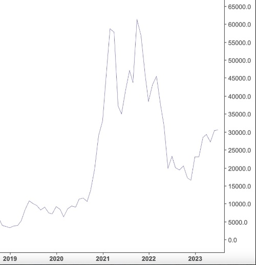
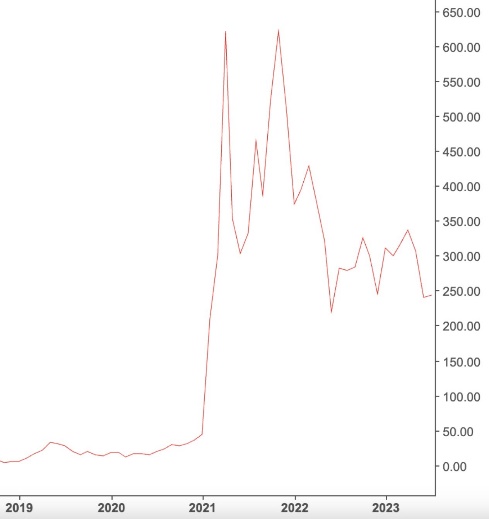
(a) Daily closing price of BTC (b) Daily closing price of BNB

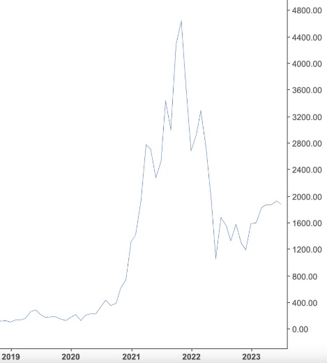
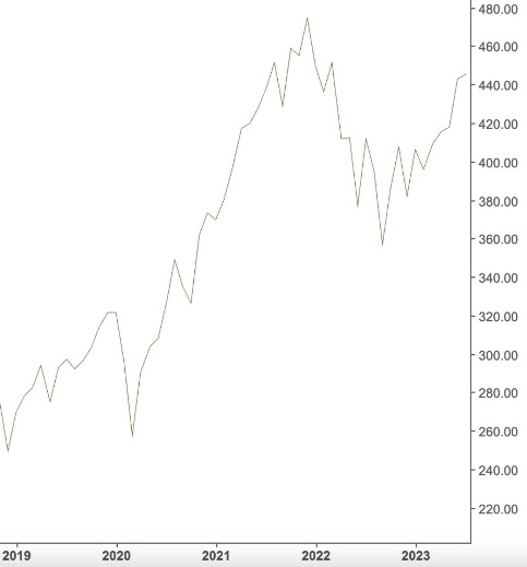
(c) Daily closing price of ETH (d) Daily closing price of S&P500

Figure 1: four Indexes’ daily closing price

According to a preliminary analysis of Figure 1, which shows the daily closing price trends of three cryptocurrencies and the S&P 500, there are shifting patterns of linkage between the US stock market and the cryptocurrency market. However, the two price evolutions have slightly different time-series trends. Although there is some correlation between the cryptocurrency market and the US stock market, this correlation is subject to alter depending on a number of variables, including policies, regulations, and the state of the world economy. Therefore, additional investigation and observation are needed for a more precise study of the link between the two markets.

Due to the existence of different trading dates between the two markets, the non-overlapping trading days, such as weekends when the stock market is closed, have been excluded from the trading data. This resulted in a final sample of 1045 time series data points.

Table 2: Description of Statistics

From Table 2, it is easy to see that the mean displays the data's average value, and the standard deviation (SD) represents the range of the series. The standard deviation of the three cryptocurrencies is larger than that of the S&P500, which indicates that the cryptocurrency market has better returns and greater volatility, according to the statistical information in the table. The maximum and lowest values represent the top and lower limits of the values for the given period of time. A greater range of return variations is also suggested by the fact that cryptocurrency has a higher maximum return than the S&P500 and a lower minimum return. All the markets display a left-skewed distribution in terms of skewness, with the S&P500 market showing the most left skewness. Both markets have kurtosis values below 0, which indicates that the distribution has a flatter peak and thinner tails than a normal distribution, meaning that more data values are concentrated around the mean and fewer data values are concentrated on the tails. Additionally, the Jarque-Bera test examines if sample data fits a normal distribution using a goodness-of-fit test. Table 2's p-value, which is close to zero at a 5% confidence level, shows that all markets' return series do not contradict the notion of a normal distribution.

Overall, these statistical measures further highlight the higher volatility and normal distribution characteristics of the cryptocurrency markets and the S&P500 market.

2.2. Methodology Choice

In the following part, stationary variables would be considered to avoid spurious regression by choosing four models: ADF, LM, Johansen Cointegration test, and Granger Causality test by using EViews, which could help conduct an empirical analysis of the correlation between the cryptocurrency market and the U.S. stock market [13,14].

2.2.1. Augmented Dickey-Fuller Test

The ADF test is used to assess whether a united root can be found in the series or if there are any problems with statical inference in this section. This information is important for determining the series' stationary state when examining the correlation between the stock market index and cryptocurrency prices. The first stage for testing unit roots is to conduct the presence of a unit root in the processes of the time span under the null hypothesis using the enhanced Dickey-Fuller test (1979) [15].

H₀: α = 0, non-stationary process

H₁: α < 0, stationary process

∆Y_t = αY_t−1+βt+ \( \sum _{j=1}^{p}γ \) ∆Y_t−j +ϵ+E (1)

2.2.2. Lagrange Multiplier-Autocorrelation Test

The Lagrange Multiplier (LM) test would be used to examine autocorrelation. These test findings can be used to determine whether or not the residuals exhibit autocorrelation. The alternative hypothesis is the presence of autocorrelation, while the null hypothesis is the absence of autocorrelation up to the chosen lag time. According to the requirements of Evans and Patterson's (1987) report, there is no autocorrelation between variables if the p-values of the t-statistic are bigger than the 5% crucial p-value [16].

H0: α = 0, there is no autocorrelation

H1: α ̸= 0, there is autocorrelation

Y_t = β₀+β₁X₁t +... +β_pX_pt +α_t (2)

αˆt = Yt −βˆt −βˆ1X1t −... −βˆpXpt (3)

2.2.3. Johansen Cointegration Test

The Johansen test is a well-liked technique for assessing cointegration and offers insights into the long-term relationship among variables [17]. It allows for more than one cointegrating relationship vector and is not accessible for the weak condition of the variables. The time series must be stationary at the initial difference in order to utilize this test. A constant term, a trend term, both of them, or neither might be present in the model, much like a unit root test. p: lag number) model for a universal VAR:

Y_t = α+β₁Y_t−1+... +β_pY_t−p +ϵ_t (4)

This could have specifications for error correction: that is, vector error correction model (VECM), which means the formula can be changed into this form:

∆Y_t = α+τ₁∆Y_t−1+... +τ_p∆Y_t−p +ϵ_t +ΘY_t−1 (5)

where ∆Y_t = Y_t −Y_t−1; Θ = parameters in matrices; τ_i = β₁β₂ ...β_p; ΘY_t−1 = error terms

The test is to consider the rank of Θ which relates to the number of independent vectors. From these conditions, we set the hypothesis to be as follows:

H₀: there is no cointegration vector.

H₁: there is one cointegration vector.

2.2.4. Granger Causality Test

The Granger causality test would be applied in the final stage to examine whether or not one-time series is significant in predicting another (Granger, 1969). Regression analysis frequently focuses on capturing correlations between variables. However, Clive Granger suggested that one way to investigate causality in economics is to measure how well one time series can predict the future values of another time series using data from the past [18]. It is crucial to remember that the use of Granger causality presupposes that the signals under study show covariance stationarity.

H0: γ1 = γ2 = ... = γi = 0 or θ1 = θ2 = ... = θi = 0, there is no causality

H1: γ1 = γ2 = ... = γi \( ≠ \) 0 or θ1 = θ2 = ... = θi \( ≠ \) 0, there is causality

Yt = α0+ \( \sum _{i=1}^{k}{α_{i}} \) Yt−i + \( \sum _{i=1}^{k}{γ_{i}} \) Xt−i +ϵt (6)

Xt = β0+ \( \sum _{i=1}^{k}{θ_{i}} \) Yt−i + \( \sum _{i=1}^{k}{β_{i}} \) Xt−i +τt (7)

where X_t, Y_t = stationary time series; ϵ, τ = residuals.

3. Empirical Results and Analysis

3.1. ADF Results

Table 3: Unit Root Test at level

A dataset spanning 4 years was used for the Augmented Dickey-Fuller (ADF) tests. LBTC (logs of Bitcoin), LETH (logs of ETH index), LBNB (logs of BNB index), and LS&P500 (logs of S&P500 index) were the variables used in the analysis. Unit roots in the series were evaluated using the ADF test. Table 3 shows the p-values for all the variables examined in this study were determined to be more than the crucial threshold of 5%, according to the results. Therefore, it may be said that all four variables exhibit non-stationary behavior, which means they have no temporal trend but rather follow a random walk pattern. It is advised to take the first difference between these variables to remedy this issue.

Table 4: Unit Root Test at First Difference

ADF tests were run on a 4-year dataset to evaluate the stationarity of the first variable. According to Table 4, all of the p-values were below the 5% critical limit, which meant that the null hypothesis was rejected. This implies that the series is non-stationary and has unit roots. The ADF test, however, revealed that all variables became stationary after the first difference of the variables. The ADF test has proven that the variables are stationary. Hence the Johansen cointegration test should be performed now that stationary behavior has been proven. This test looks at whether the variables' initial differences show any long-term correlations.

3.2. LM Test Results

For the LM tests in this investigation, a 4-year dataset was employed. The Serial Correlation LM test was used specifically to evaluate autocorrelation. The objective of the test was to assess if the variables exhibit any autocorrelation up to a certain lag, with the alternative hypothesis arguing that autocorrelation does exist up to the predetermined lag. After reviewing the results in Table 5, it was discovered that all p-values above the 5% cutoff point. As a result, we were unable to rule out the null hypothesis, proving that the variables' autocorrelation is not very strong. Furthermore, it can be deduced from these results that the error term does not exhibit serial correlation. Therefore, the Johansen cointegration test may be performed in the following step.

Table 5: LM-Autocorrelation Test

3.3. Johansen Cointegration Test Results

Table 6: Johansen Cointegration Test of Three Cryptocurrencies

The statistical result of the Maximum Eigenvalue test for BTC, as shown in Table 6, is 16.43, which is higher than the critical value of 14.26. Additionally, the Trace test's statistical value of 16.80 is greater than the crucial threshold of 15.49. As a result, we can rule out the null hypothesis that there is no cointegration, proving that Bitcoin and the S&P 500 do in fact, cointegrate. Similarly to this, the Maximum Eigenvalue test for ETH has a statistical value of 26.55, which is higher than the critical value of 14.26. Furthermore, the Trace test's statistical value is 26.57, which is higher than the crucial limit of 15.49. As a result, we may draw the conclusion that ETH and S&P500 cointegrate. All of the statistical results of the Maximum Eigenvalue test, however, for BNB, are lower than the critical value of 14.26 at 13.66. Additionally, the Trace test's statistical value is 13.72, which is below the crucial criterion of 15.49. We do not discover any proof of cointegration between BNB and S&P500 as a result.

3.4. Granger Causality Test Results

Table 7: Granger Causality Test of Three Cryptocurrencies

Based on Table 7, the empirical results of BTC show the unidirectional Granger Cause for these two variables. The causality direction is the S&P500 stock index Granger Cause BTC but not vice versa. It means that the S&P500 stock index is the leading BTC for the analysis time. Similarly, for ETH, it is easy to see that there exists a unidirectional Granger Cause between them. The causality direction is the S&P500 stock index Granger Cause ETH but not vice versa. It means that the S&P500 stock index has an influence on ETH during that time. However, in BNB, the empirical results find no Granger Cause for the two indexes.

4. Conclusions

All in all, cryptocurrencies have continued to gain popularity with more and more people around the world and are going across a broad economic spectrum recently. In this study, some properties of cryptocurrencies and the correlation between traditional investment options, such as stocks, indicate their importance for the financial field. To begin, literature reviews help to build a basic understanding of its history. Second, explore some statistical data on the subject and demonstrate 4 tests to contribute to the information about them. Lastly, identify and analyze these tests to enable to obtain some significant findings and implications.

From these results found of the previous test, the empirical results show that United States stock market indexes have significantly strong causality within BTC and ETH, which gives a chance for the investors to promote their investment strategies and potential possibilities of earning them in relation to looking movement in the U.S. economy. The influence of the United States economy would create a movement of the economy to cause BTC and ETH. However, the United States is affected by BNB prices, which means that BNB prices have causality and are statistically significant for affecting the stock market index of the U.S. This may be because the cryptocurrency has not had an original currency, but the transactions are made by dollar currency, which means they would have relationship or causality between them. This change in the bond markets would offer investors important signals about the global economy’s direction. Because the bond markets are deep by nature, it is possible to analyze changes in global economic conditions, which means the causality and relationship between them should be paid more attention in this direction.

Cryptocurrency is a quite new topic and exerts more and more influence on the economy daily. Such as, macroeconomic variables, like the GDP or interest rate, would be related and have causality affection in the future. Furthermore, with the strengthening of technological development, the necessity of changing business and central banks of the countries would be tending to use blockchain technologies instead of conventional digital money. Therefore, the awareness of cryptocurrency will increase progressively soon. In the end, theoretically, this paper enriches the existing literature available on cryptocurrency, especially because it considers more kinds of cryptocurrency. Most of the results are consistent and show the relationship between cryptocurrency and U.S. stock markets.

References

[1]. K. Keogh J. G A., Rejeb. Cryptocurrencies in modern finance: a literature review. Rejeb, 20 (1):93–118, 2021.
[2]. Ying Wang Vasileios Kallinterakis. Do investors herd in cryptocurrencies – and why? Research in International Business and Finance, 50:240–245, 2019.
[3]. S Nakamoto. Bitcoin: A peer-to-peer electronic cash system. 2008.
[4]. Donncha Kavanagh and Paul Dylan-Ennis. Cryptocurrencies and the emergence of blockocracy. The Information Society, 36(5):290–300, 2020.
[5]. Lykke Øverland Bergsli, Andrea Falk Lind, Peter Molnar, and Michał Polasik. Forecasting´ volatility of bitcoin. Research in International Business and Finance, 59:101540, 2020.
[6]. Paraskevi Katsiampa. Volatility estimation for bitcoin: A comparison of GARCH models? Economics Letters, 158:3–6, 2017.
[7]. Andrew Urquhart Larisa Yarovaya Shaen Corbet, Brian Lucey. Cryptocurrencies as a financial asset: A systematic analysis. International Review of Financial Analysis, 62:182–199, 2019.
[8]. J.I Chikwira, C.; Mohammed. The impact of the stock market on liquidity and economic growth: Evidence of volatile market. Economies, 11:125, 2023.
[9]. Saeed Sazzad Jeris, A. S. M. Nayeem Ur Rahman Chowdhury, Mst. Taskia Akter, Shahriar Frances, and Monish Harendra Roy. Cryptocurrency and stock market: bibliometric and content analysis. Heliyon, 8(9), 2022.
[10]. Cem Kartal and Umran Ozturk Can. Analysis of the correlation between cryptocurrencies and us 10-year treasury bond index with granger causality test. Journal of Management and Economics Research, 20(2):274 – 291, 2022.
[11]. Semra Boga Melih Sefa Yavuz, Gozde Bozkurt. Investigating the market linkages between¨ cryptocurrencies and conventional assets. Emerging Markets, 10(2), 2022.
[12]. Igor Makarov and Antoinette Schoar. Price discovery in cryptocurrency markets. AEA Papers and Proceedings, 109:97–99, 2019.
[13]. Yuxuan Du. Research on the linkage between the cryptocurrency market and the u.s. stock market. Finance, 11(3), 2021.
[14]. Li J Akinci, E. Bitcoin and stock market indexes causality. 2018.
[15]. David A. Dickey and Wayne A. Fuller. Distribution of the estimators for autoregressive time series with a unit root. Journal of the American Statistical Association, 74(366):427–31, 1979.
[16]. David M. Lilien Engle, Robert F. and Russell P. Robins. Estimating time varying risk premia in the term structure: The arch-m model. Econometrica, 55(2):391–407, 1987.
[17]. Johansen Søren. Statistical analysis of cointegration vectors. Journal of Economic Dynamics and Control, 12(23):231–254, 1998.
[18]. C. W. J Granger. Investigating causal relations by econometric models and cross-spectral methods. Econometrica, 37(3):424–38, 1969.
Cite this article
Yang,G. (2024). Quantitative Analysis of the Relationship Between Cryptocurrency Market and U.S. Stock Market Performance. Advances in Economics, Management and Political Sciences,97,122-131.
Data availability
The datasets used and/or analyzed during the current study will be available from the authors upon reasonable request.
Disclaimer/Publisher's Note
The statements, opinions and data contained in all publications are solely those of the individual author(s) and contributor(s) and not of EWA Publishing and/or the editor(s). EWA Publishing and/or the editor(s) disclaim responsibility for any injury to people or property resulting from any ideas, methods, instructions or products referred to in the content.
About volume
Volume title: Proceedings of the 2nd International Conference on Financial Technology and Business Analysis
© 2024 by the author(s). Licensee EWA Publishing, Oxford, UK. This article is an open access article distributed under the terms and
conditions of the Creative Commons Attribution (CC BY) license. Authors who
publish this series agree to the following terms:
1. Authors retain copyright and grant the series right of first publication with the work simultaneously licensed under a Creative Commons
Attribution License that allows others to share the work with an acknowledgment of the work's authorship and initial publication in this
series.
2. Authors are able to enter into separate, additional contractual arrangements for the non-exclusive distribution of the series's published
version of the work (e.g., post it to an institutional repository or publish it in a book), with an acknowledgment of its initial
publication in this series.
3. Authors are permitted and encouraged to post their work online (e.g., in institutional repositories or on their website) prior to and
during the submission process, as it can lead to productive exchanges, as well as earlier and greater citation of published work (See
Open access policy for details).