1. Introduction

A stock price is the present valuation of a particular share of a company that can be purchased or sold on the stock market. It mirrors the amount at which interested investors are willing to buy in a specified time frame. The price may fluctuate throughout the trading day, dependent on a diversity of factors, including market conditions, performance of the company, investor attitude, and numerous others. Researchers have employed various methods to try to predict stock prices with relative accuracy. For example, they used News Articles [1], Candlestick Charts [2], and Crossover Simple Moving Averages (SMA) [3] to predict stock price movement. However, because of the complex nature of the stock market, it's still difficult to predict a completely convincing result. Nowadays, more developed techniques come out, which could make more accurate predictions to a large extent. Among them, machine learning is one of the representatives. It offers the ability to analyze a vast amount of data and capture the complicated features of the stock market that traditional methods miss. For this project, the method of machine learning is used to capture the features of the stock market and predict stock prices using the historical data from Edwards Lifesciences Corporation (EW). This is an essential and valuable subject that helps investors and analysts make informed decisions, develop strategies, and manage risks effectively.

2. Methodology

2.1. Encryption of Data

The dataset was collected from Kaggle. But in fact, the data is downloaded from finance.yahoo.com, which shows the historical stock prices of Edwards Lifesciences Corporation (EW) from 2000 to 2017. By observing the first rows of our data, it is composed of seven variables, including date (the date of the stock data), open (the Opening price of the stock on a given day), high (the highest price reached during the day), low (the lowest price during the day), close (the closing price of the stock on a given day), adj-close (the adjusted closing price, which accounts for corporate actions), and volume (the number of shares traded during the day). There are 4392 observations and no missing data, which are great for our subsequent exploratory data analysis and model building. However, after checking the type of each variable, the Date variable is categorical while all others are numerical. Since this paper aims to predict the stock price, regression models are appropriate to fit quantitative data. Thus, it’s more convenient to convert all categorical variables to numerical form.

2.2. Data Conversion

Let’s begin to make a data conversion. The chosen method is to choose a reference date and convert each date to the number of days since that reference date. The following steps are needed to complete our data conversion.

Convert the date column to the date time format using the pd.to_datetime () function that is used to convert a column to a date time format, which allows us to convert these dates to numerical values later.

stock_data['Date'] = pd.to_datetime(stock_data['Date'])

Choose the first date in our data as our reference date.

reference_date = stock_data['Date'].min()

Convert the column to the number of days since the chosen reference date.

stock_data['Date2'] = (stock_data['Date'] - reference_date).dt.days

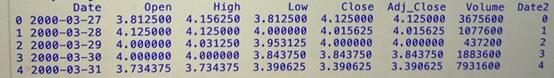
Figure 1: Statistics of the updated dataset

By checking the first rows of our data again, a new variable has been added called Date2 which is numerical.

2.3. Visualization

After data conversion, the next step is the visualization. But before doing that, it’s important to define the response and predictors. Compared to the closing price, the adjusted closing price is more appropriate to be the response, since it accounts for dividends and stock splits, which provides a more accurate representation of the stock’s value over time. Thus, the adjusted closing price is chosen as our response, and other remaining variables: date, open, high, low, close, and volume, as our predictors. Then, visualization can be used to explore the underlying features of data.

Firstly, a time series plot of the adjusted closing price can be created to check whether the price could change over time.

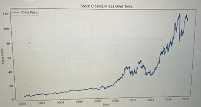
Figure 2: Stock Closing Price Over Time

According to the plot, the overall trend of adjusted closing prices is upward. During that process, starting from 2014, the upward process is evident. In 2017, the price rarely decreased sharply from 120 to 80 due to some reasons. However, it recovered to the normal in 2018. Therefore, although sometimes the adjusted closing price could decrease, the overall trend is upward. Secondly, plot the histogram to explore the distribution of our response.

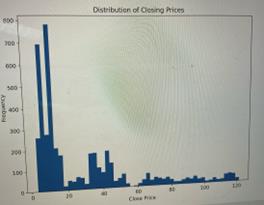
Figure 3: Distribution of Closing Prices

The graph shows a distribution that appears to be positively skewed, which means there are more occurrences of lower adjusted closing prices and fewer occurrences of higher prices. The peak of the histogram, which is the most common price, ranges from 4 to 16.

After exploring the response, the highest price is an interesting term that deserves to be analyzed. For example, what is the highest price throughout the trading days? The boxplot is chosen to draw a box plot to observe the observation of highest prices each trading day.

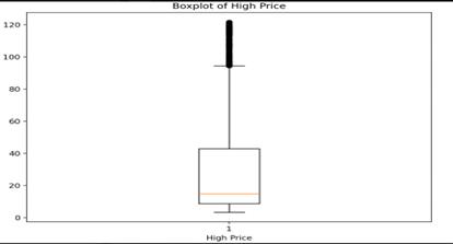
Figure 4: Boxplot of Highest Prices

The boxplot shows that the high prices of the stock have a median value of around 20, with most values falling between 10 and 40. There are many high-value outliers, which indicates some days, the stock price was significantly higher than usual.

Finally, plot a correlation plot, which is a convenient way to visualize each relationship between variables.

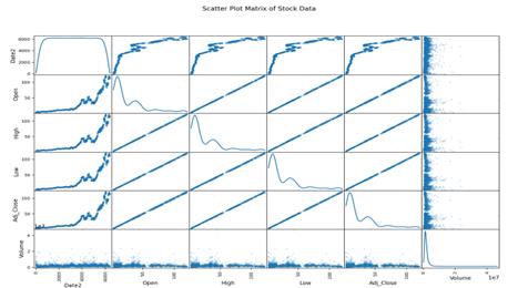
Figure 5: Scatter Plot Matrix of Stock Data

According to the plot, the variables open, high, low, and adj_close show a clear upward trend over time (date2). This indicates that the prices have generally increased over time covered by the data. In addition, there are strong linear relationships between open, high, low, and adj_close prices. However, the volume in the plot doesn’t show a clear trend over time and any strong relationship with all price variables, which indicates that the volume has remained relatively stable, and the prices are not influenced by it.

2.4. Model Selection

Let's begin to build our models. Since the outcome is quantitative, models should be used for regression cases. Here, some common regression models are selected: linear regression model [4], random forest model [5], K-nearest neighbours model [6], and support vector machines model [7]. Before fitting these models to the data, it’s important to split data into two parts: a training set and a testing set. The training set is used to train and fit the models. Then, the performance of models needs to be tested using the testing set, and the best-performing one is chosen based on testing RMSE (root mean squared error). A lower RMSE represents a better fit of our model to the data, which means the predicted values calculated by the model are closer to the actual values. Thus, the best-performing model will have the minimal value of testing RMSE.

Following the process above, each model is fitted to the training set and evaluated using the testing set. Finally, the values of RMSE are calculated for each model.

Table 1: RMSE for each model

According to the table, the random forest model performs the best because it has the lowest value of testing RMSE. It’s not surprising because this model always performs well. After all, it is non-parametric and doesn't assume a parametric form, which makes it more flexible. In addition, it’s also normal that K-Nearest neighbors and support vector machines perform badly. For KNN, it relies heavily on the distance metric to find the nearest neighbors. Hence, as the number of features increases, the data points will become sparse, which will lead to poor performance. For SVM, it performs badly possibly because of the improper feature scaling. Since the support vector machines model is sensitive to the scale of input features, it could perform badly if the features are not normalized. The only surprising point is the low RMSE value of the linear regression model. The nature of the stock market is generally volatile and nonlinear. Thus, the final performance of the linear regression model may not be as expected.

Figure 6: Statistics of the dataset

By observing the first rows of our data again, for Edwards Lifesciences Corporation (EW), the fluctuation range between prices on different trading days is very small, which may lead to a higher performance of the linear regression model.

3. Limitations

Admittedly, some places limit the overall accuracy of our models. For instance, an excessively low RMSE value might show that the model is overfitting the training data, which could lead to poor performance on unseen data. Besides, according to the correlation plot, the strong correlations among independent variables may lead to multicollinearity, which might inflate standard errors and produce inaccurate results. Finally, due to the limitation of our data, it’s hard to completely capture the trend of the stock market, because it only provides basic data such as the open price, highest price, and lowest price of each trading day. Although linear regression and other methods can be applied using this data and perform relatively well, the limitations of the dataset restrict the comprehensive analysis necessary for accurate real-life stock price prediction.

4. Conclusion

In short, this project has been meaningful in demonstrating the application of different machine learning models in stock price prediction and their effectiveness. Linear regression and random forest models performed well and were able to provide valuable predictions and analyses for practical investment decisions. Although the KNN model is not as effective as the first two, it is still a useful tool for understanding the data. These results not only enhance our understanding of stock price prediction but also provide a solid theoretical foundation and methodological guidance for practical applications. However, that is just the beginning. There are many places for improvement in the future. For instance, additional data variables could be included, such as Market Sentiment Indicators [8], Macroeconomic Indicators [9], Technical indicators [10], News and Events, and Company Fundamentals [11]. In addition, adopting more advanced models to more accurately fit the data of the stock market, such as Long Short-Term Memory (LSTM) [12], convolutional Neural Network (CNNs) [13], and Gated Recurrent Units (GRUs). [14] In a word, although our project has a lot of restrictions, it provides a solid foundation for using more developed techniques to predict stock prices later.

References

[1]. Gidófalvi, Győző. "Using News Articles to Predict Stock Price Movements." Department of Computer Science and Engineering, University of California, San Diego, June 15, 2001.
[2]. Lee, K.H., and G.S. Jo. "Expert System for Predicting Stock Market Timing Using a Candlestick Chart." In Expert Systems with Applications, vol. 16, no. 4, May 1999, pp. 357-364.
[3]. Kardile, Rucha, Trishna Ugale, and Sachi Nandan Mohanty. "Stock Price Predictions using Crossover SMA." 2021 9th International Conference on Reliability, Infocom Technologies and Optimization (Trends and Future Directions) (ICRITO), Amity University, Noida, India, Sep 3-4, 2021.
[4]. Hope, Thomas M. H. (2020). Linear regression. In Machine Learning: Methods and Applications to Brain Disorders (pp. 67-81).
[5]. Biau, Gerard. (2024). Analysis of a Random Forests Model. Universite Pierre et Marie Curie – Paris VI, LSTA & LPMA.
[6]. Zhang, Zhongheng. (2016). Introduction to machine learning: k-nearest neighbors. Annals of Translational Medicine, 4(11), 218.
[7]. Kecman, V. (2005). Basics of machine learning by support vector machines. In Real World Applications of Computational Intelligence (pp. 49-103).
[8]. Beer, Francisca., & Zouaoui, Mohamed. (2013). Measuring stock market investor sentiment. The Journal of Applied Business Research.
[9]. Ali, Rafaqat, Muhammad Abrar ul Haq, and Shafqut Ullah. "Macroeconomic Indicators and Stock Market Development." vol. 5, no. 9, 2015.
[10]. Oriani, Felipe Barboza, and Guilherme P. Coelho. "Evaluating the impact of technical indicators on stock forecasting." In 2016 IEEE Symposium Series on Computational Intelligence (SSCI). IEEE.
[11]. Ozlen Serife. "The Effect of Company Fundamentals on Stock Values." European Researcher, vol. 71, no. 3-2, 2014. Ishik University, Erbil, Iraq.
[12]. Roondiwala, Murtaza, Harshal Patel, and Shraddha Varma. "Predicting Stock Prices Using LSTM." International Journal of Science and Research (IJSR), ISSN (Online): 2319-7064, 2015. Index Copernicus Value: 78.96 | Impact Factor: 6.391.
[13]. Lopez Pinaya, Walter Hugo, Sandra Vieira, Rafael Garcia-Dias, and Andrea Mechelli. "Convolutional Neural Networks." In Machine Learning, 2020, pp. 173-191.
[14]. Rahman, Mohammad Obaidur, Md. Sabir Hossain, Ta-Seen Junaid, Md. Shafiul Alam Forhad, and Muhammad Kamal Hossen. "Predicting Prices of Stock Market using Gated Recurrent Units (GRUs) Neural Networks." IJCSNS International Journal of Computer Science and Network Security, vol. 19, no. 1, January 2019.
Cite this article
Huang,Z. (2024). Predicting Edwards Lifesciences’ Stock Prices Using Machine Learning Model. Advances in Economics, Management and Political Sciences,105,76-82.
Data availability
The datasets used and/or analyzed during the current study will be available from the authors upon reasonable request.
Disclaimer/Publisher's Note
The statements, opinions and data contained in all publications are solely those of the individual author(s) and contributor(s) and not of EWA Publishing and/or the editor(s). EWA Publishing and/or the editor(s) disclaim responsibility for any injury to people or property resulting from any ideas, methods, instructions or products referred to in the content.
About volume
Volume title: Proceedings of the 3rd International Conference on Financial Technology and Business Analysis
© 2024 by the author(s). Licensee EWA Publishing, Oxford, UK. This article is an open access article distributed under the terms and
conditions of the Creative Commons Attribution (CC BY) license. Authors who
publish this series agree to the following terms:
1. Authors retain copyright and grant the series right of first publication with the work simultaneously licensed under a Creative Commons
Attribution License that allows others to share the work with an acknowledgment of the work's authorship and initial publication in this
series.
2. Authors are able to enter into separate, additional contractual arrangements for the non-exclusive distribution of the series's published
version of the work (e.g., post it to an institutional repository or publish it in a book), with an acknowledgment of its initial
publication in this series.
3. Authors are permitted and encouraged to post their work online (e.g., in institutional repositories or on their website) prior to and
during the submission process, as it can lead to productive exchanges, as well as earlier and greater citation of published work (See
Open access policy for details).