1. Introduction

When making investment decisions, it is necessary to analyze securities and portfolio management to help investors choose good investments. For a long time, investors analyzed stocks solely on the basis of their fundamentals and recent earnings performance. However, the market environment and conditions are constantly changing, and investors need to adjust their investment strategies in time according to new information. So, in the current volatile market environment, there has been a shift away from a single focus on individual stocks to a broader consideration of the risk and return profile of different portfolios. This is where modern portfolio theory (MPT) comes into play, providing a framework for investors to allocate capital across various assets and construct optimal portfolios [1-2]. Since investors face great uncertainty in selecting stocks, risk preferences depend on each individual investor and are usually represented in modern portfolio theory by setting constraints. Therefore, figuring out how to balance high returns with low risks is definitely a key area of focus in financial research.

Over the decade many researchers have conducted research on portfolio and diversification. For instance, Fischer and Robert introduced the global CAPM balance model and discussed how to apply the global asset allocation model to the actual investment decision to solve the two major problems in the traditional model that the expected return is hard to estimate, and the optimal portfolios are too sensitive to expected return assumptions [3]. Philippe took the international bond portfolio as an example; a simulation method is proposed to evaluate the reliability of mean-variance analysis in portfolio optimization by making a comparison between the performance of the ex-post optimal portfolio and the world bond index and the US bond index [4]. Myles presented Markowitz's contributions to modern portfolio theory from a simple perspective and provided an in-depth look at the complex mathematical/statistical models commonly associated with discussions of the theory [5]. Niranjan used the Sharpe single index model to construct the optimal portfolio and compared it with Markowitz's mean-variance model [6]. However, most of the previous studies compared the differences between the two models in theory, but rarely applied the Markowitz model and the index model to select assets and construct portfolios for optimal planning simulation.

Given the description mentioned above, this article aims to carry out a real-world examination of the contrast between improving the Markowitz investment portfolio and enhancing the Index investment portfolio. Based on the stock assets of the US stock market, this paper will go through the process of data processing, model building, and data visualization, and compare the effects of the two models in optimizing the portfolio with the specific result data.

2. Data

The research collated approximately two decades of S&P 500 returns, spanning from May 1, 2004, to June 1, 2024. This dataset was augmented with data for six individual stocks, each drawn from three distinct sectors, as well as an instrument representing the risk-free rate, the 5-year treasury yield. The data were sourced from Yahoo Finance. The S&P 500 index was chosen as a proxy for market performance due to its status as a comprehensive, diversified, and universally acknowledged indicator. The subsequent Table 1 presents the selected six stocks and their respective details.

Table 1: Stock ticker symbols in portfolios

Then the daily data were consolidated into monthly observations to mitigate the influence of non-Gaussian effects and reduce the time of calculation. The monthly return was computed by difference return.

Additionally, the residual return was calculated, which equates to the return minus the sum of the risk-free rate the product of the beta coefficient, and the difference between the market return and the risk-free rate. Subsequently, the annual average return, annual standard deviation, beta, and alpha were computed with the Excel-inserted functions based on the excess return, and the residual standard deviation was derived from the residual return. With these computations in place, the correlation matrix among the six stocks and the index was calculated using an Excel function.

The Table 2 shows that Apple and NVIDIA have the highest annual average return during the 20 years, at 34.01% and 41.85% respectively. The return volatility of all stocks is greater than the volatility of the Sharpe index, and the largest volatility is for NVIDIA and Ford.

BAC and JPM have the strongest correlation with the Sharpe index, which may mean that the stock performance of financial services companies is closely related to the performance of the market. Meanwhile, there is a strong positive correlation between Bank of America Corporation (BAC) and JPMorgan Chase & Co. (JPM) with a correlation coefficient of 0.804329. This means that when BAC's stock price rises, JPM's stock price is likely to follow suit, and vice versa (See Table 3).

Table 2: Descriptive statistics of the seven assets

Table 3: Correlation matrix of the seven assets

3. Method

In this section, there will be a delineation of two methodologies employed in venture capital: the Markowitz approach and the Index model. These frameworks facilitate the assembly of diverse investment portfolios, catering to the varying objectives of investors, including the construction of minimum variance portfolios and maximum Sharpe ratio portfolios.

The following key concepts are used in the model:

Expected value of asset return: Investors' expectations of future returns.

Variance and standard deviation of asset returns: A statistical measure of asset risk; the smaller the variance, the lower the risk.

Correlation between assets: correlation between returns of different assets, low correlation can diversify risk.

Efficient frontier of the portfolio: The frontier formed by all possible portfolios in the risk-return plane, representing the maximum possible return for different levels of risk.

Capital Market Line (CML): denotes the existence of a portfolio between the market portfolio and the risk-free asset that provides the highest expected return for each level of risk [7].

Sharpe Ratio: Measures the ratio of the excess return (the portion of the portfolio that exceeds the risk-free rate) to the overall risk (usually expressed in standard deviation).

3.1. Markowitz Model

Harry Markowitz introduced what is known as the Markowitz model, or Modern Portfolio Theory (MPT), in the year 1952. The model provides a quantitative method for investors to construct and evaluate portfolios with the aim of maximizing expected returns for a given level of risk or minimizing risk for a given expected return.

The core idea of the Markowitz model is to treat the risk and return of a portfolio as a weighted average of the risks of the assets in the entire portfolio. It hypothesizes that investors are risk-averse, in the sense that they tend to choose portfolios that are less risky for the same expected return [8-9].

Drawing upon the foundational assumptions, the Markowitz model is capable of accurately determining the desired outcomes for investors through the employment of two key equations:

where:

E(Rp​) is the expected return of this portfolio

𝑤𝑖 is the weight of asset i

E(Ri​) is the expected return of asset i

where:

\( {{σ_{p}}^{2}} \) is the variance of the portfolio

𝑤𝑖 is the weight of asset i

\( {{σ_{i}}^{2}} \) is the variance of asset i

\( {σ_{ij}} \) is the covariance of asset i and asset j

The advantage of the Markowitz model lies in its comprehensive consideration of the risk and return of each asset in the portfolio, as well as their mutual relationship, so as to achieve risk diversification and return maximization more effectively. Compared with other models, it provides a more comprehensive and personalized framework, enabling investors to construct tailored optimal investment strategies according to their own risk preferences.

3.2. Index Model

Following the establishment of the Markowitz portfolio analysis model, its shortcomings became apparent. A significant limitation is the complexity and unwieldiness of its computation, which is further encumbered by the extensive number of estimations required, thereby diminishing computational efficiency and precision. To address these issues, Professor William Sharpe developed an alternative analytical model that simplifies the analysis of security portfolios while maintaining user-friendliness. This model is the Single Index Mode, usually referred to as the Capital Asset Pricing Model (CAPM). It was developed independently in the 1960s by William Sharpe, John Lintner, and Jan Mossin. The model provides a simplified way to evaluate the expected return of a security or portfolio in comparison to its systematic risk [10].

The core idea of CAPM is that the expected return of a security or portfolio is related to the expected return of the market as a whole and is proportional to its sensitivity to market risk. This sensitivity is often referred to as beta (β), which is a way to measure the volatility of a security or portfolio relative to the entire market. The basic formula of CAPM is as follows:

Where:

E(Ri​) is the expected return on a security or portfolio.

Rf​ is the risk-free rate.

𝛽𝑖 is the beta of the security or portfolio

𝐸(𝑅𝑚) is the expected return of the market portfolio

The advantages of the index model for constructing an optimal portfolio lie in its simplicity, low cost, and wide diversification, which enables investors to track market performance with low fees and achieve stable returns over the long term. Compared with the complexity and the need for active management of the Markowitz model, the index model provides a more straightforward and easy-to-implement strategy for investors who seek average market performance and moderate risk appetite.

4. Result

In this research, five constraints are also added to obtain the portfolio's optimal solution in various cases. Using these five constraints, the policies and regulations of different national markets and the investment preferences of most investors in the real world can be well simulated. In this scenario, the parallel examination and the subsequent differentiation between the two models exhibit greater harmony and feasibility.

1. This extra optimisation constraint is intended to mimic the rules of Regulation T set by FINRA. The stockbroker is permitted to enable their clients to have positions, which at least 50% financed by the equity in the client’s account:

2. This accessional constraint is formulated to mimic certain predefined “box” constraints on the allocation of weights, as specified by the client.

3. A “free” problem, devoid of any extra optimization restrictions, is presented to demonstrate the general shape of the feasible portfolio region and the efficient frontier.

4. The supplementary optimization restrain is purposefully crafted to replicate the standard limitations prevalent in the United States' mutual fund sector, which includes the ban on short selling for American open-ended mutual funds.

5. Lastly, to investigate if incorporating the comprehensive index into the portfolio influences it favorably or unfavorably, it introduces another optimization constraint:

4.1. Markowitz Model

By using the programming solver function of Excel, each asset weight and return rate, standard deviation, and Sharpe ratio data of the optimal portfolio obtained by the minVar strategy and maxSharpe strategy under five different constraints are found (See Table 4).

Table 4: Minimum variance portfolio and maximum shape portfolio in MM under five constraints

The information presented in the table leads to the following conclusion:

1. In the minVar strategy in all constraints, the weight of the SPX index is zero. However, in the max Sharpe strategy, the weight of SPX is the highest under all constraints (except the fifth constraint, which requires SPX weight to be 0), indicating that it is a very effective asset in terms of risk-adjusted return and can significantly improve the Sharpe ratio of the portfolio

2. Under the condition of allowing short selling, the weight of JPM in the max Sharpe strategy is in the range of -34.59% to -32.08%, which means that the price of JPM is expected to decline and the operation of shorting JPM is taken

3. In the minVar strategy under all constraints, the weight of BAC is the highest (31.55%-32.3%), and the weight of F is the second highest (26.3%-27.69%). By checking the correlation coefficient matrix, it is found that this is because the correlation between these two stocks and other assets is low. It can play a better role in diversifying risks in the portfolio, thus reducing the overall variance

4. The returns and standard deviations of the minVar strategy under the five constraints are relatively stable, with Sharpe ratios ranging from 147.85% to 150.94%. The returns and standard deviations of the max Sharpe strategy fluctuate widely, with Sharpe ratios ranging from 95.68% to 110.76%.

Then, the CAL was drawn by the return and standard deviation on constraint 3. Through running the solver table, a figure of the Minimal Variance Frontier, Efficient Frontier, and Inefficient Frontier of the portfolio under the five constraints was drawn (See Figure 1).

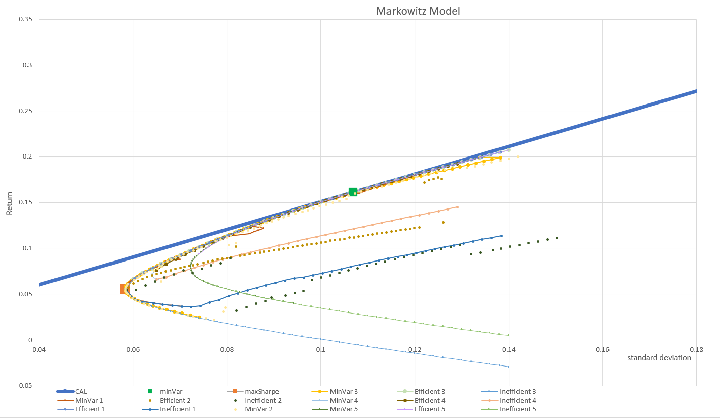
Figure 1: CAL and Minimal Variance Frontier, Efficient Frontier and Inefficient Frontier in MM under five constraints

4.2. Index Model

By using the programming solver function of Excel, each asset weight and return rate, standard deviation, and Sharpe ratio data of the optimal portfolio obtained by the minVar strategy and maxSharpe strategy under five different constraints are found.

The information presented in the table leads to the following conclusion:

1. SPX occupies the main weight in the minimum variance (minVar) strategy and the maximum Sharpe ratio (maxSharpe) strategy under most constraints, especially in the minVar strategy in constraints 1 to 4, the weight is close to or more than 95%. While the weight in the maxSharpe strategy is close to or more than 100%.

2. The weight of AAPL, NVDA and AMZN in constraint 5 increases significantly

3. JPM has a negative weight in the maxSharpe strategy under all constraints, especially in constraints 1 and 3 with a weight of -2.27% and in constraint 2 with a weight of -1.56%, showing short operation.

4. The return and standard deviation of minVar strategy under constraints 1 to 4 are relatively stable, with the return between 6.74% and 6.76%, the standard deviation around 6.71%, and the Sharpe ratio between 100.55% and 100.62%. The return and standard deviation in constraint 5 increase significantly, with a return of 10.26%, a standard deviation of 15.25%, and a Sharpe ratio of 67.30%.

The maxSharpe strategy has fewer volatile returns and standard deviations under constraints 1 to 4, with returns ranging from 6.53% to 6.63%, standard deviations ranging from 6.55% to 6.63%, and Sharpe ratios ranging from 99.63% to 100.01%. The return and standard deviation in constraint 5 also increase, and the return is 9.81%, the standard deviation is 14.91%, and the Sharpe ratio is 65.82% (See Table 5).

Table 5: Minimum variance portfolio and maximum shape portfolio in IM under five constraints

Then, the CAL was drawn by the return and standard deviation on constraint 3. Through running the solver table, a figure of the Minimal Variance Frontier, Efficient Frontier, and Inefficient Frontier of the portfolio under the five constraints was drawn (See Figure 2).

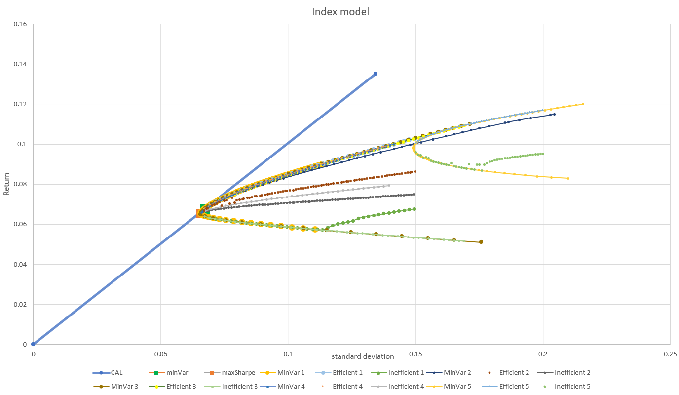
Figure 2: CAL and Minimal Variance Frontier, Efficient Frontier and Inefficient Frontier in IM under five constraints

By comparing the conclusions of using the Markowitz model and the index model to construct the optimal portfolio, this study finds that the weight distribution of different stocks is more balanced under the Markowitz model, especially under the minimum variance strategy, the effect of risk diversification is more significant. The index model, on the other hand, relies more on the weight allocation of a single stock, especially on the SPX, which is heavily weighted under most of the constraints, probably due to the high representativity and stability of the SPX in the market. Under both models, portfolio returns, and standard deviations fluctuate with different constraints, but in general, the Sharpe ratio is higher for the Markowitz model, indicating that its risk-adjusted returns are higher. However, the portfolio returns, and standard deviation of the index model are relatively stable, but they fluctuate greatly under constraint 5, and the Sharpe ratio is slightly lower than that of the Markowitz model.

5. Conclusion

The results of this paper show that both Markowitz model and index model have advantages and disadvantages in portfolio optimization, and investors should pick the applicable model that consistent with their own risk preference and market environment. The Markowitz model is suitable for investors who pursue risk diversification and personalized investment strategies, while the index model is more suitable for investors who pursue average market returns and low costs. In addition, there are differences in the portfolio allocation and risk-return characteristics of the two models under different constraints, so investors should choose and adjust according to their own situation and market environment.

References

[1]. Putra, I. K. A. A. S., & Dana, I. M. (2020). Study of optimal portfolio performance comparison: Single index model and Markowitz model on LQ45 stocks in Indonesia stock exchange. American Journal of Humanities and Social Sciences Research (AJHSSR), 4(12), 237-244.
[2]. Fabozzi, F. J., Gupta, F., & Markowitz, H. M. (2002). The legacy of modern portfolio theory. The journal of investing, 11(3), 7-22.
[3]. Black, F., & Litterman, R. (1992). Global portfolio optimization. Financial analysts journal, 48(5), 28-43.
[4]. Jorion, P. (1992). Portfolio optimization in practice. Financial analysts journal, 48(1), 68-74.
[5]. Mangram, M. E. (2013). A simplified perspective of the Markowitz portfolio theory. Global journal of business research, 7(1), 59-70.
[6]. Mandal, N. (2013). Sharpe’s single index model and its application to construct optimal portfolio: an empirical study. Great Lake Herald, 7(1), 1-19.
[7]. Feldman, D., & Reisman, H. (2003). Simple construction of the efficient frontier. European Financial Management, 9(2), 251-259.
[8]. Guo, Q. (2022, April). Review of research on markowitz model in portfolios. In 2022 7th International Conference on Social Sciences and Economic Development (ICSSED 2022) (pp. 786-790). Atlantis Press.
[9]. Hali, N. A., & Yuliati, A. (2020). Markowitz model investment portfolio optimization: a review theory. International Journal of Research in Community Services, 1(3), 14-18.
[10]. Shah, C. A. (2015). Construction of optimal portfolio using sharpe index model & camp for bse top 15 securities. International Journal of Research and Analytical Reviews, 2(2), 168-178.
Cite this article
Zheng,J. (2024). Markowitz Model and Index Model: A Comparative Study of Constructing Optimal Portfolios. Advances in Economics, Management and Political Sciences,99,23-32.
Data availability
The datasets used and/or analyzed during the current study will be available from the authors upon reasonable request.
Disclaimer/Publisher's Note
The statements, opinions and data contained in all publications are solely those of the individual author(s) and contributor(s) and not of EWA Publishing and/or the editor(s). EWA Publishing and/or the editor(s) disclaim responsibility for any injury to people or property resulting from any ideas, methods, instructions or products referred to in the content.
About volume
Volume title: Proceedings of ICFTBA 2024 Workshop: Finance in the Age of Environmental Risks and Sustainability
© 2024 by the author(s). Licensee EWA Publishing, Oxford, UK. This article is an open access article distributed under the terms and
conditions of the Creative Commons Attribution (CC BY) license. Authors who
publish this series agree to the following terms:
1. Authors retain copyright and grant the series right of first publication with the work simultaneously licensed under a Creative Commons
Attribution License that allows others to share the work with an acknowledgment of the work's authorship and initial publication in this
series.
2. Authors are able to enter into separate, additional contractual arrangements for the non-exclusive distribution of the series's published
version of the work (e.g., post it to an institutional repository or publish it in a book), with an acknowledgment of its initial
publication in this series.
3. Authors are permitted and encouraged to post their work online (e.g., in institutional repositories or on their website) prior to and
during the submission process, as it can lead to productive exchanges, as well as earlier and greater citation of published work (See
Open access policy for details).