1. Introduction

In the financial market, constructing an optimized investment portfolio is an essential task. In the year 1952, a significant breakthrough was made in the field with the introduction of Modern Portfolio Theory (MPT) by Harry Markowitz [1]. It was shown that the overall performance of a portfolio carries more weight than that of an individual stock [2]. MPT providing investors with a systematic way to balance risk and return.

Currently, the rolling window model is widely used in portfolio construction, regarding as an effective method. Studies have demonstrated that the rolling window model effectively manages the dynamic characteristics of time series data, which means portfolio risk and return can be optimized [3]. However, although many studies have combined rolling window models with portfolio construction, relevant research is still limited. For example, many existing studies focus on specific markets or asset classes and lack systematic evaluations of the model's stability under different market conditions [4-5]. Additionally, many studies have certain limitations in the application of the method and fail to fully consider various constraints in practical operations [6].

This study proposes a new method to address the mentioned concerns, which combines mean-variance analysis with a rolling window model in order to optimize portfolios. Firstly, five stocks (AAPL, JPM, JNJ, XOM, PG) were selected to ensure diversity and representativeness of the portfolio. The stock data covers 100 trading days from February 2nd, 2024, to June 27th, 2024. Adjusted closing prices from Yahoo Finance were used in this study to calculate daily returns. By using rolling window, the size of the window was set to 70 days, and it moved forward by one day at each iteration. For each rolling window, this study calculates the annualized average anticipated returns and covariance matrix for the next day. These forecasts are used to identify the optimal investment portfolio weights that maximize the Sharpe ratio. Subsequently, the performance of optimized investment portfolios in the last 30 days is evaluated in this study. To assess the robustness of this approach, results from different window sizes (60 days and 80 days) are compared. In addition, this study compares the cumulative returns of optimizing investment portfolios with the S&P 500 index and analyzes the effectiveness of the proposed method. This study further evaluates the precision of the predictions by determining the mean squared error (MSE) between the forecasted values and the real returns. Through this comprehensive approach, this paper aims to assist investors in making better investment decisions.

2. Data

The adjusted closing prices of the stock data utilized in this paper are obtained from Yahoo Finance (https://finance.yahoo.com/). This paper selected five stocks (AAPL, JPM, JNJ, XOM, PG) to ensure diversity and representativeness in the portfolio (See Table 1). This selection helps to diversify investment risk and allows us to observe the performance of different industries under the same market conditions. And chose the yield on the 3-month U.S. Treasury bill (^IRX). These data cover the adjusted closing prices for each stock, which more accurately reflect the impact of dividend payments and corporate actions (such as stock splits). The stock data spans from Feb 2nd, 2024, to Jun 27th, 2024, lasting 100 trading days. This period provides a recent market snapshot, offering a solid foundation for our analysis.

From the Table 2, it is easy to find that Apple Inc. (AAPL) has the highest mean return at 0.12%, while Johnson & Johnson (JNJ) has the lowest mean return at 0.04%. Exxon Mobil Corporation (XOM) has the highest standard deviation of returns, suggesting its greater volatility. Procter & Gamble Co. (PG) exhibits the lowest standard deviation, which points to more stable returns. Under the same market conditions, different stocks exhibit distinct returns and volatilities. This also reflects the representativeness of the stocks chosen in this study.

Table 1: Selected stocks

Table 2: Descriptive statistics of five stocks

3. Methods

3.1. Rolling Window Model

The rolling window model employs a dynamic adjustment strategy. It’s constantly updating model parameters over various time periods allows the portfolio to respond to market changes [7], which reflects market fluctuations and trend changes in real-time. The size of the rolling window can be tailored to specific needs, enabling adaptation to various market environments. By smoothing data, it reduces the influence of daily fluctuations on the model.

In this study, the rolling window size is set to 70 days, advancing one day at a time. The average daily returns from days 1 to 70 are used to predict the return on day 71, and the predicted covariance matrix is calculated. The next window is formed using data from days 2 to 71, and this process continues in a similar manner. Ultimately, the study derives the predicted annual average returns and covariance matrix for days 71 to 100. The optimal weights are calculated based on the daily data from the past 30 days.

3.2. Mean-Variance Model

In modern portfolio management, the mean-variance model is a foundational theory, which was developed by Harry Markowitz. Due to its explicit consideration of both expected return and portfolio risk, the mean-variance model is suitable for portfolio construction. It allows for an optimal balance between the two. Also, the model analyzes the correlation between assets to quantify the benefits of diversification, aiding in reducing overall portfolio risk.

The anticipated portfolio return, \( \text{E}(\text{R}_{\text{P}}) \) , is determined by combining the expected returns of each individual asset, taking into account their respective weights. The weight assigned to the i-th asset in the portfolio is denoted as \( \text{w}_{\text{i}} \) , while its expected return is represented by \( \text{r}_{\text{i}} \) .

\( \text{E}(\text{R}_{\text{P}})\text{=}\text{W}^{\text{T}}\text{R=}\sum _{\text{i}}^{} \text{w}_{\text{i}}\text{r}_{\text{i}} \) (1)

The expected return variance of the portfolio, \( \text{σ}_{\text{P}}^{\text{2}} \) , is determined by utilizing the covariance matrix of asset returns [8]. \( \text{w}_{\text{i}} \) and \( \text{w}_{\text{j}} \) represent the weights assigned to asset i and asset j correspondingly. The covariance between \( \text{r}_{\text{i}} \) and \( \text{r}_{\text{j}} \) is \( \text{cov}(\text{r}_{\text{i}}\text{r}_{\text{j}}) \) .

\( \text{σ}_{\text{P}}^{\text{2}}\text{=var}(\sum _{\text{i}}^{} \text{w}_{\text{i}}\text{r}_{\text{i}}\text{ })\text{=}\sum _{\text{ij}}^{} \text{w}_{\text{i}}\text{w}_{\text{j}}\text{cov}(\text{r}_{\text{i}}\text{r}_{\text{j}}) \) (2)

The portfolio's Sharpe ratio serves as a measure for evaluating returns in relation to risk and can be computed using the following formula [9]. The anticipated return of the portfolio is indicated as \( \text{R}_{\text{p }} \) , whereas the risk-free rate is symbolized by \( \text{R}_{\text{f}} \) [10]. The standard deviation \( \text{σ}_{\text{p}} \) is equivalent to the square root of its variance.

\( \text{Sharpe Ratio= }\frac{\text{R}_{\text{p }}\text{ - }\text{R}_{\text{f}}}{\text{σ}_{\text{p}}} \) (3)

4. Result

This paper downloads historical price data for five stocks from different industries, calculates daily returns for 100 trading days, and uses a rolling window method to determine the optimal investment portfolio weights for each day to maximize the Sharpe ratio.

Firstly, the method for predicting returns and covariance matrix involves calculating the average daily returns and covariance matrix over a rolling window of 70 days, and then annualizing them to obtain the predicted values for future one-day returns and covariance matrix. The following day's predicted values are obtained by sliding the window forward by one day, until predictions are obtained for all thirty subsequent days. The following Figure 1 shows a comparison between the non-annualized forecasted values and the actual values for the next thirty days.

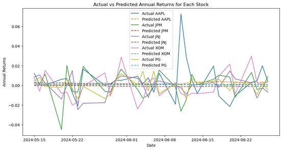
Figure 1: Returns Comparison

Here is the Mean Squared Error (MSE) between the predicted values and the actual values in Table 3:

Table 3: MSE between the predicted values and the actual values

On average, the difference between predicted and actual returns is small, as indicated by the low mean squared error (MSE) value, which suggests that using rolling window calculations to determine average returns is an accurate method for capturing trends in stock returns.

Among them, Procter & Gamble (PG) and Johnson & Johnson (JNJ) have lower MSE values, indicating higher prediction accuracy. In contrast, Apple (AAPL) has a higher MSE value, suggesting relatively lower prediction accuracy.

Then, obtain the yield of the 3-month US Treasury bill as the risk-free rate, define a function for maximum Sharpe ratio and constraints, use optimization algorithms to calculate optimal weights within each rolling window, and store them in a DataFrame. Finally, compute and plot the cumulative returns of this optimized investment portfolio and the S&P 500 index for comparison. Below is a comparison chart of cumulative returns.

From Figure 2, it can be seen that the optimized investment portfolio initially performed well, closely following the trend of the Standard & Poor's 500 Index. However, in the subsequent duration, its performance significantly lagged behind the S&P 500 index and exhibited greater volatility. In comparison, the Standard & Poor's 500 Index showed a more stable performance with some fluctuations but overall presented an upward trend, resulting in significantly higher cumulative returns compared to the optimized investment portfolio.

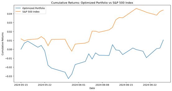
Figure 2: Cumulative return comparison plot (window size:70)

5. Robust Test

Setting the window size to 80 days, the cumulative returns of the optimized portfolio (blue line) and S&P 500 index (orange line) are initially close at the beginning. In the early stages, the optimized portfolio performs slightly better, but after a few days, they gradually converge. Ultimately, the S&P 500 index continues its upward trend and achieves significantly higher cumulative returns than the optimized portfolio. Related results are shown in the following Figure 3.

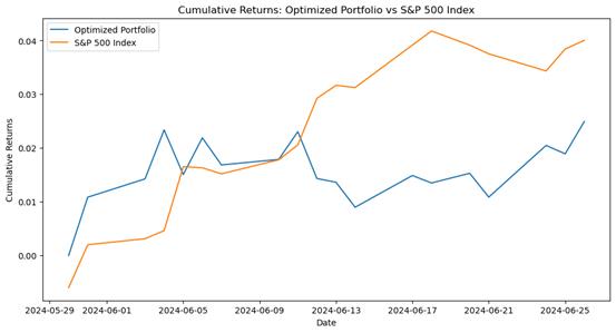
Figure 3: Cumulative return comparison plot (window size:80)

Setting the window size to 60 days, the initial cumulative returns of the optimized portfolio which were similar to S&P 500 index. In the first few days, the performance of the S&P 500 index just slightly outperformed the optimized portfolio. However, the S&P 500 index continued to rise, and its cumulative returns significantly surpassed those of the optimized portfolio in the later period. Related results are shown in the following Figure 4.

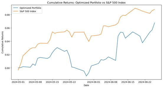
Figure 4: Cumulative return comparison plot (window size:60)

By comparing different window sizes (80 days, 60 days, and 70 days), the performance trends of optimized investment portfolios can be observed under different window sizes. Across all window sizes, the cumulative returns of optimized investment portfolios have not significantly surpassed the S&P 500 index, although they may have come close or slightly exceeded it during certain periods. This suggests that there is still room for improvement in the long-term performance of optimized investment portfolios.

6. Conclusion

The article explored a method to optimize dynamic investment portfolios by combining the rolling window approach and mean-variance model to maximize risk-adjusted returns. This paper used adjusted closing price data from five stocks (AAPL, JPM, JNJ, XOM, PG) obtained from Yahoo Finance with the aim of improving return prediction accuracy and optimizing portfolio weights. Annualized average returns and covariance matrices within a 70-day period were calculated through the rolling window approach, which were updated daily. This method demonstrated high precision in prediction. The mean-variance model was applied in this study to calculate the optimal portfolio weights using these predictions, with the objective of maximizing the Sharpe ratio. The optimized portfolio performed well initially. But its long-term performance did not outperform the S&P 500 index. Valuable insights into the potential and limitations of using dynamic optimization techniques in portfolio management for investors in financial markets were provided by the findings.

This study provides a practical portfolio optimization method. But it has limitations. Analyzing a limited dataset may not capture complex market conditions. It also doesn’t include diversified asset behaviors. Further research can be conducted by expanding the range of assets and exploring different market environments. To verify and enhance the robustness of the proposed method and improve prediction accuracy, advanced machine learning algorithms, such as LSTM, can be used. This may lead to better portfolio performance and provide new directions for future research.

References

[1]. Markowitz, H. (1952). Portfolio selection. The Journal of Finance, 7(1), 77-91.
[2]. Elton, E. J., Gruber, M. J., & Mei, J. (1994). Cost of capital using a fundamental factor model. Journal of Financial Economics, 35(1), 1-22.
[3]. Campbell, J. Y., & Thompson, S. B. (2008). Predicting excess stock returns out of sample: Can anything beat the historical average? The Review of Financial Studies, 21(4), 1509-1531.
[4]. DeMiguel, V., Garlappi, L., & Uppal, R. (2009). Optimal versus naive diversification: How inefficient is the 1/N portfolio strategy? The Review of Financial Studies, 22(5), 1915-1953.
[5]. Jagannathan, R., & Ma, T. (2003). Risk reduction in large portfolios: Why imposing the wrong constraints helps. The Journal of Finance, 58(4), 1651-1683.
[6]. Ledoit, O., & Wolf, M. (2004). Honey, I shrunk the sample covariance matrix. The Journal of Portfolio Management, 30(4), 110-119.
[7]. Zivot, E., & Wang, J. (2003). Rolling analysis of time series. In Modeling Financial Time Series with S-Plus, 507-552
[8]. Barry, C. B. (1974). Portfolio Analysis Under Uncertain Means, Variances, and Covariances. The Journal of Finance, 29(2), 515–522.
[9]. Sharpe, W. (1998). The Sharpe Ratio (Fall 1994). In P. Bernstein & F. Fabozzi (Ed.), Streetwise: The Best of The Journal of Portfolio Management, 169-178.
[10]. Weil, P. (1989). The equity premium puzzle and the risk-free rate puzzle. Journal of Monetary Economics, 24(3), 401-421.
Cite this article
Chen,P. (2024). Portfolio Optimization Based on Rolling Window Using 5 Stocks. Advances in Economics, Management and Political Sciences,90,91-97.
Data availability
The datasets used and/or analyzed during the current study will be available from the authors upon reasonable request.
Disclaimer/Publisher's Note
The statements, opinions and data contained in all publications are solely those of the individual author(s) and contributor(s) and not of EWA Publishing and/or the editor(s). EWA Publishing and/or the editor(s) disclaim responsibility for any injury to people or property resulting from any ideas, methods, instructions or products referred to in the content.
About volume
Volume title: Proceedings of the 3rd International Conference on Financial Technology and Business Analysis
© 2024 by the author(s). Licensee EWA Publishing, Oxford, UK. This article is an open access article distributed under the terms and
conditions of the Creative Commons Attribution (CC BY) license. Authors who
publish this series agree to the following terms:
1. Authors retain copyright and grant the series right of first publication with the work simultaneously licensed under a Creative Commons
Attribution License that allows others to share the work with an acknowledgment of the work's authorship and initial publication in this
series.
2. Authors are able to enter into separate, additional contractual arrangements for the non-exclusive distribution of the series's published
version of the work (e.g., post it to an institutional repository or publish it in a book), with an acknowledgment of its initial
publication in this series.
3. Authors are permitted and encouraged to post their work online (e.g., in institutional repositories or on their website) prior to and
during the submission process, as it can lead to productive exchanges, as well as earlier and greater citation of published work (See
Open access policy for details).