1. Introduction

The dynamic and complex nature of financial markets requires sophisticated portfolio management and optimization strategies. Two essential models that have significantly shaped the field of portfolio theory are the Markowitz model, also known as the mean-variance model, and the index model. Each of these models brings a unique set of principles and methodologies aimed at improving portfolio performance by balancing risk and return.

The Markowitz model, introduced by Harry Markowitz in his groundbreaking 1952 article "Portfolio Selection," is the way investors thought about diversification and risk [1] By quantitatively evaluating the trade-off between risk and return, the Markowitz model provides a framework for constructing an optimal portfolio that maximizes the expected return for a given level of risk or, conversely, the expected risk for a given level of return [2]. This model works on the principle that an investor can achieve an optimal portfolio through careful asset allocation based on expected returns, variances and covariances. Markowitz's brilliance lies in his mathematical rigor, which allows him to define an efficient term for the sum of portfolios with the expected return for a certain risk. In contrast, the index model popularized by William Sharpe simplifies the computational complexity associated with Markowitz by requiring a relationship between individual returns and a common index. The main index model is the assumption that the returns of individual securities are linearly related to the returns of a market index, such as the S&P 500. This model introduces the concept of beta, a more sensitive factor to market movements, which facilitates a more streamlined and practical approach to portfolio optimization. By breaking down total risk into systematic and unsystematic components, the index model allows investors to factor in market risk, assuming that idiosyncratic risks can be removed.

The comparative analysis of the Markowitz Model and the Index Model in portfolio management is not merely an academic exercise but a practical investigation into their real-world applications and effectiveness. The Markowitz Model, with its comprehensive and precise approach, is often lauded for its theoretical robustness. However, its reliance on extensive and often unavailable data for covariances, as well as the computational intensity of deriving the efficient frontier, can be seen as limitations in practical scenarios. The model originally incorporated iso-mean and iso-variance surfaces for proving portfolio optimization [3]. On the other hand, the Index Model, with its simplification and reliance on readily available market data, offers a more accessible and less computationally demanding alternative [4]. Single-index modeling is widely applied in, for example, econometric studies as a compromise between too restrictive parametric models and flexible but hardly estimable purely nonparametric models [5] Yet, this model's assumptions about market efficiency and the linearity of returns may not hold true in all market conditions, potentially leading to suboptimal portfolio choices [6,7].

This paper aims to explore and compare the usage of the Markowitz Model and the Index Model in constructing and managing investment portfolios. Through a detailed examination of their theoretical underpinnings, computational methodologies, and practical implications, we seek to understand the strengths and weaknesses of each model. Furthermore, we will assess their performance in various market conditions, drawing on empirical data and case studies to provide a comprehensive evaluation.

The comparative analysis will also consider the impact of modern advancements in computational finance and data availability on the applicability and efficiency of these models. As the financial landscape evolves with the advent of big data analytics, machine learning, and algorithmic trading, the relevance and adaptability of traditional models like those of Markowitz and Sharpe are of paramount interest. This investigation will provide insights into how these foundational models can be integrated with contemporary techniques to enhance portfolio optimization strategies.

In conclusion, this article aims to bridge the difference between theoretical models and actual investment strategies by offering a nuanced comparison of the Markowitz Model and the Index Model. By critically analyzing their respective methodologies, assumptions, and real-world applications, our goal is to provide ongoing portfolio management and proactive insights to investors seeking to make the best investment decisions in an increasingly complex and volatile economic environment [8].

2. Construction of models

In the area of financial economics, the concepts of the efficient frontier, inefficient frontier, and minimum variance frontier hold pivotal importance in the construction and optimization of investment portfolios. These theoretical constructs, rooted in modern portfolio theory, provide investors with the tools and frameworks necessary to balance risk and return, ultimately guiding them toward more informed and strategic investment decisions. Each of these frontiers—efficient, inefficient, and minimum variance—offers unique insights into the risk-return trade-off and has distinct implications for portfolio management.

In this article, we will only use a single-index model with S&P500 Index, there are also more complex index models such as two-index models [9].

2.1. The Efficient Frontier

The efficient frontier is the cornerstone of portfolio theory. It was first introduced by Harry Markowitz in his seminal 1952 article, “Portfolio Selection.” It represents the set of optimal portfolios with a certain level of risk or the lowest risk that offer the highest expected return or a given expected return. An efficient frontier involves showing portfolios on a risk-return graph, where the x-axis represents risk (the standard deviation of portfolio returns is usually measured) and the y-axis represents expected return.

Portfolios that lie on the efficient frontier are considered optimal because they maximize returns for a specific level of risk. Conversely, for a given expected return, they minimize risk. The efficient frontier is generally ascending, reflecting the positive relationship between risk and return. The slope and shape of the efficient frontier can provide valuable information about market conditions and the potential benefits of diversification [10].

The Inefficient Frontier in contrast to the efficient frontier, the inefficient frontier represents portfolios that do not optimize the risk-return trade-off. These portfolios either have higher levels of risk for a given return or lower returns for a given level of risk compared to those on the efficient frontier. Essentially, any portfolio that lies below of the efficient frontier is always seen as inefficient.

Portfolios on the inefficient frontier may be suboptimal due to various reasons, such as lack of diversification, poor asset allocation, or erroneous investment strategies. Investors aiming to improve their portfolio performance should seek to move from the inefficient frontier towards the efficient frontier by optimizing their asset allocation and leveraging diversification benefits.

2.2. The Inefficient Frontier

In contrast to the efficient frontier, the inefficient frontier represents portfolios that do not optimize the risk-return trade-off. These portfolios either have higher levels of risk for a given return or lower returns for a given level of risk compared to those on the efficient frontier. Essentially, any portfolio that lies below or to the right of the efficient frontier is considered inefficient.

Portfolios on the inefficient frontier may be suboptimal due to various reasons, such as lack of diversification, poor asset allocation, or erroneous investment strategies. Investors aiming to improve their portfolio performance should seek to move from the inefficient frontier towards the efficient frontier by optimizing their asset allocation and leveraging diversification benefits.

2.3. The Minimum Variance Frontier

The minimum variance frontier is a specific subset of the efficient frontier, focusing exclusively on portfolios that minimize risk. It is constructed by identifying the portfolio combinations that yield the lowest possible variance (or standard deviation) for all possible expected returns. The portfolio with the absolute lowest variance on this frontier which also means the global minimum variance portfolio.

The minimum variance frontier is significant because it highlights the role of diversification in risk reduction. Even without considering expected returns, constructing portfolios that lie on the minimum variance frontier ensures that risk is minimized given the set of available assets. This is especially useful for risk-averse investors who prefers stability and capital preservation than high returns.

2.4. Data source

We used 10 stocks, as can be seen in Figure 1: Amazon.com, Inc., Figure 2: Apple Inc., Figure 3: Citrix Systems, Inc., Figure 4: JPMorgan Chase & Co., Figure 5: Berkshire Hathaway Inc., Figure 6: The Progressive Corporation, Figure 7: United Parcel Service, Inc., Figure 8: FedEx Corporation, Figure 9: J.B. Hunt Transport Services, Inc., and Figure 10: Landstar System, Inc. Their stock price graphs as below:

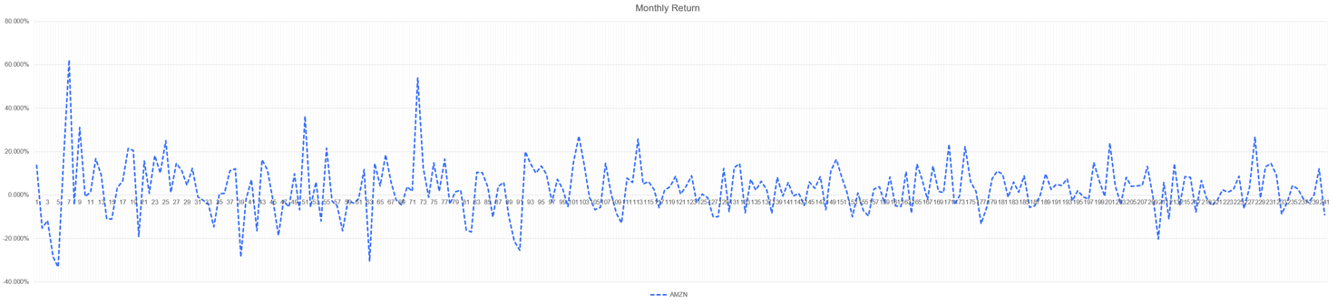
Figure 1: Amazon Inc.

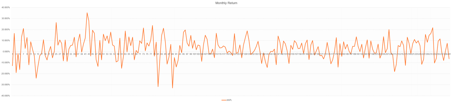
Figure 2: Apple Inc.

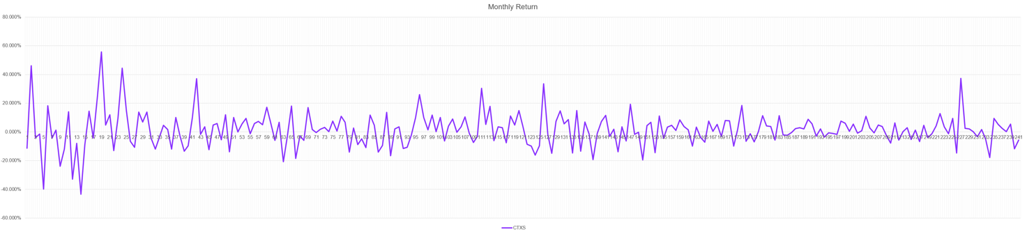
Figure 3: Citrix Systems, Inc.

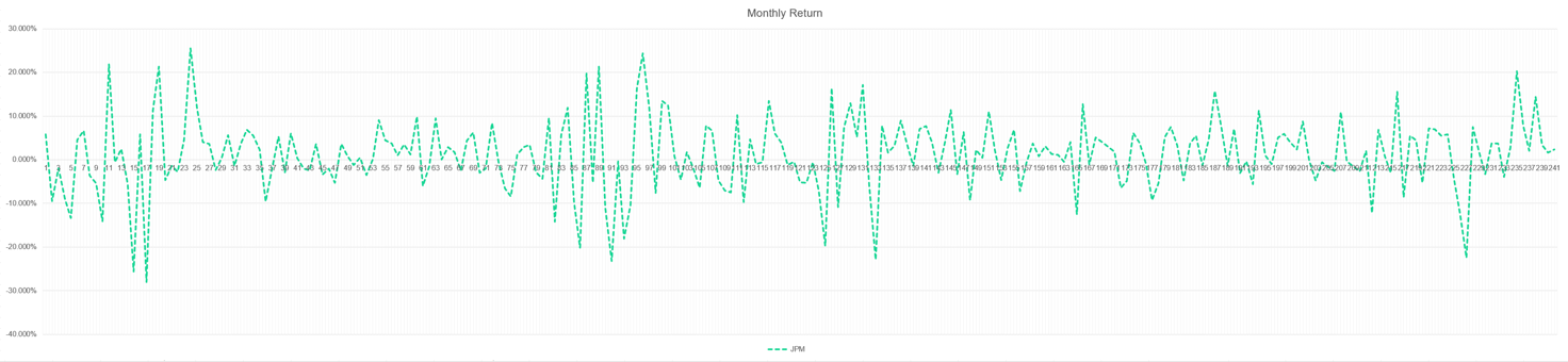
Figure 4: JPMorgan Chase & Co.

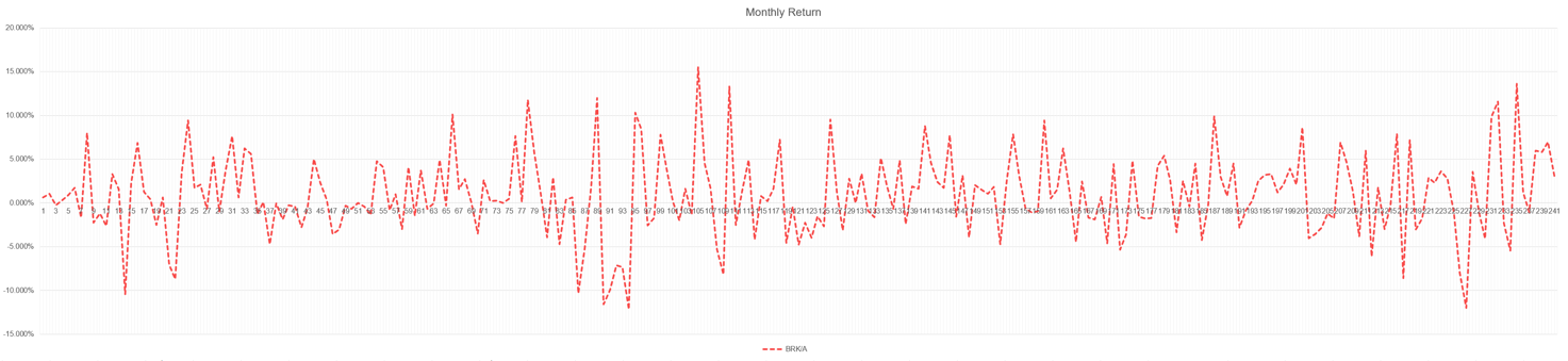
Figure 5: Berkshire Hathaway Inc.

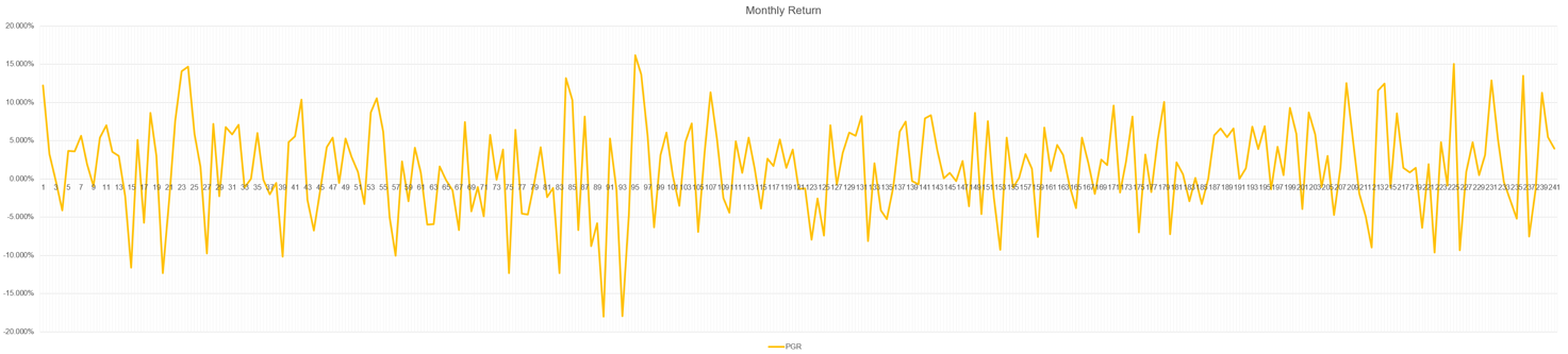
Figure 6: The Progressive Corporation.

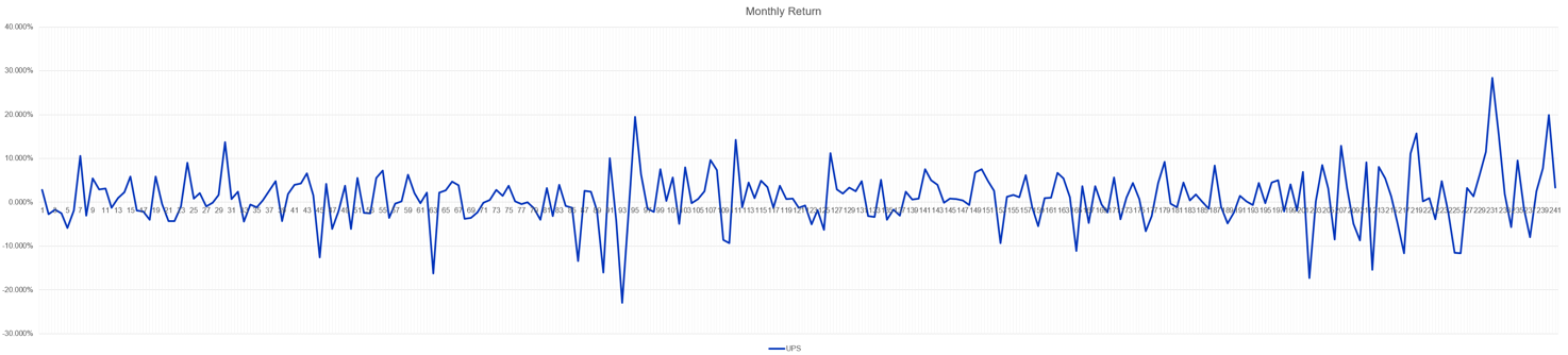
Figure 7: United Parcel Service, Inc.

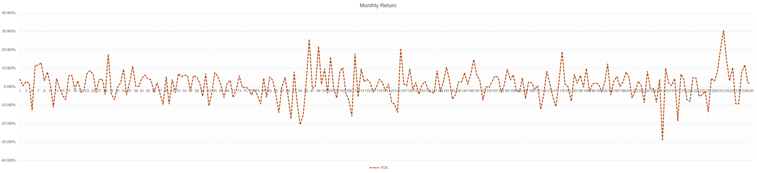
Figure 8: FedEx Corporation.

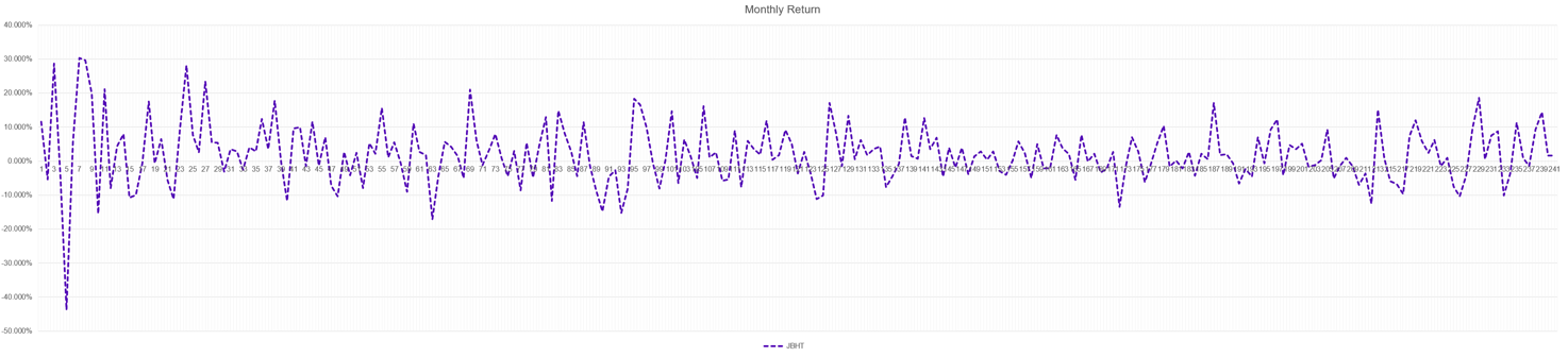
Figure 9: J.B. Hunt Transport Services.

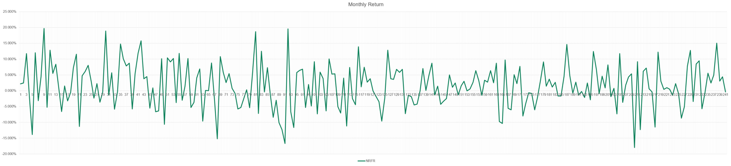
Figure 10: Landstar System, Inc.

3. Data Processing

We began by selecting ten representative stocks from various sectors to ensure a diversified portfolio. The chosen stocks. Historical daily closing prices for these stocks were collected over a five-year period to provide a comprehensive dataset for analysis.

Before we start data processing, we first need to pre-process our data, which is divided into 2 parts: Data cleaning, and Normalization:

Data Cleaning: The raw data was cleaned to remove any anomalies, such as missing values or outliers. Missing values were handled by linear interpolation, and outliers were identified using the z-score method and subsequently smoothed to minimize their impact on the analysis.

Normalization: To ensure comparability across stocks with different price ranges and volatilities, the data was normalized. This involved transforming the price data into logarithmic returns, which mitigates the impact of extreme values and stabilizes the variance.

We calculated the correlation matrix of the 10 stocks:

\( \text{∑=}\frac{\text{1}}{\text{n-1}}\text{(X-}\bar{\text{X}}\text{)}^{\text{T}}\text{(X-}\bar{\text{X}}\text{)} \) (1)

Where \( \text{X} \) \( \text{X} \) is the matrix of stock returns and 𝑋 is the matrix of mean returns. The resulting correlation matrix, illustrated in Figure 11, highlighted higher correlations among stocks within the same sector, indicating shared market influences. is the matrix of stock returns and \( \bar{\text{X}} \)

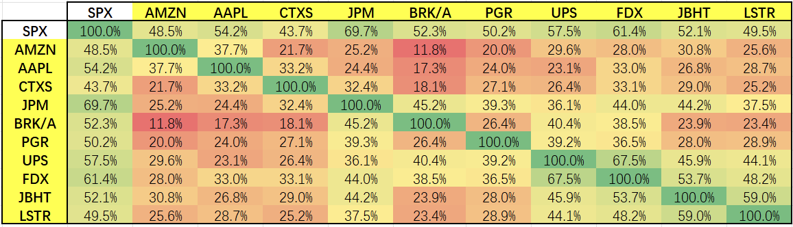
Figure 11: The correlation matrix of the stocks.

We noticed that due to production chain and other reasons, stocks of companies in the same sector have a relatively higher correlation coefficient.

For the Index Model, we calculated their coefficients as Figure 12:

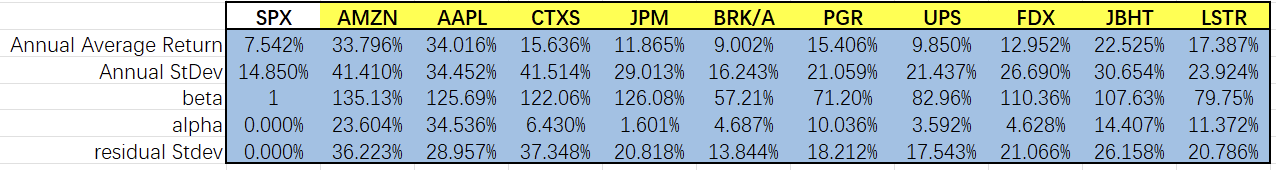
Figure 12: Coefficients for Index Model.

The formula of Index Model:

\( \text{R=α+β*}\text{R}_{\text{M}}\text{+e } \) (2) \( \text{R=α+β*}\text{R}_{\text{M}}\text{+e } \)

\( \text{R} \) \( \text{R} \) means the return of a stock, \( \text{α} \) \( \text{α} \) represents the stock's excess return independent of the market, 𝑅 𝑀 is the return on the market portfolio, and 𝑒 is the idiosyncratic return of stock, representing the component of the stock's return that is independent of the market. [11]. represents the stock's excess return independent of the market, \( \text{R}_{\text{M}} \) is the return on the market portfolio, and \( \text{e} \) \( \text{e} \)

Under the same portfolio, in contrast of the two models, MM give us a higher expected return, and higher Sharpe, although their standard deviations remain almost the same (Figure 13):

Figure 13: Weights, returns, and Standard deviations for one portfolio.

3.1. Portfolio Constraints

We set 5 constraints to simulate the portfolio constraints people might have in real life:

Con1: The sum of the absolute values ​​of all weights is less than 2.

Con2: The absolute value of any weight is less than 1.

Con3; Free problem, no constraints.

Con4: Weight of any stock is more than 0.

Con5: Weight of risk-free investment is 0.

\( \text{con1: }\sum _{\text{i=1}}^{\text{n}} |\text{w}_{\text{i}}|\text{≤2 }\text{ } \) (3) \( \text{con1: }\sum _{\text{i=1}}^{\text{n}} |\text{w}_{\text{i}}|\text{≤2 }\text{ } \)

\( \text{con2: }|\text{w}_{\text{i}}|\text{≤1 } \) (4) \( \text{con2: }|\text{w}_{\text{i}}|\text{≤1 } \)

\( \text{con3:no constraints } \) (5) \( \text{con3:no constraints } \)

\( \text{con4: }\text{w}_{\text{i}}\text{≥0 } \) (6) \( \text{con4: }\text{w}_{\text{i}}\text{≥0 } \)

\( \text{con5: }\text{w}_{\text{1}}\text{=0 } \) (7) \( \text{con5: }\text{w}_{\text{1}}\text{=0 } \)

The result of minimum variance portfolio comes as follow:

Table 1: MiniVar and MaxSharpe portfolios of Markowitz Model

Table 2: MiniVar and MaxSharpe portfolios of Index Model

We notice that under some of the constraints, the difference of the two models cannot be ignored.

3.2. Results and Analysis

The minimum variance portfolio results under different constraints were compared for both models. Figures 14 and 15 show the portfolio allocations and their respective returns and standard deviations. It was observed that under certain constraints, the differences between the models became significant.

3.3. Frontiers

We plotted the efficient, inefficient, and minimum variance frontiers for both models. Figures 14 and 15 demonstrate these frontiers, revealing that while the efficient frontiers were similar, the inefficient and minimum variance frontiers showed noticeable differences under various constraints. [10].

With frontiers drown, we compared these two models, the valid frontiers are similar, but under some circumstances, the frontiers are more like scattered points, and these frontiers are quite different:

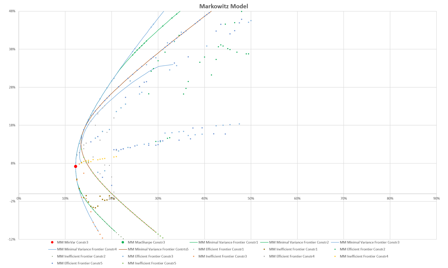
Figure 14: Frontiers of Markowitz Model.

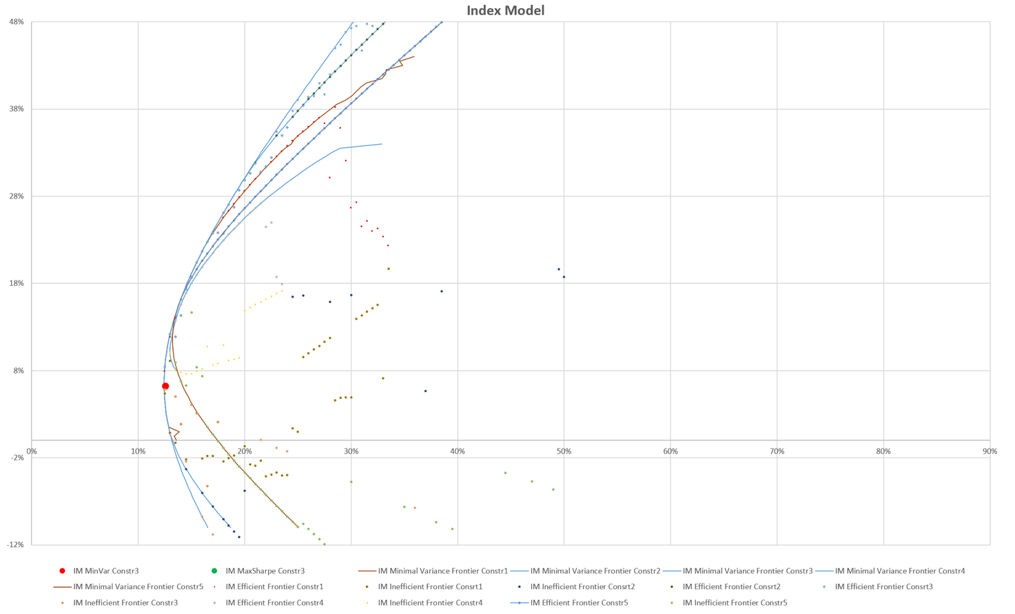
Figure 15: Frontiers of Index Model.

3.4. Robustness Analysis

To measure the robustness, we calculated the excessive return, and excessive variance of the frontiers:

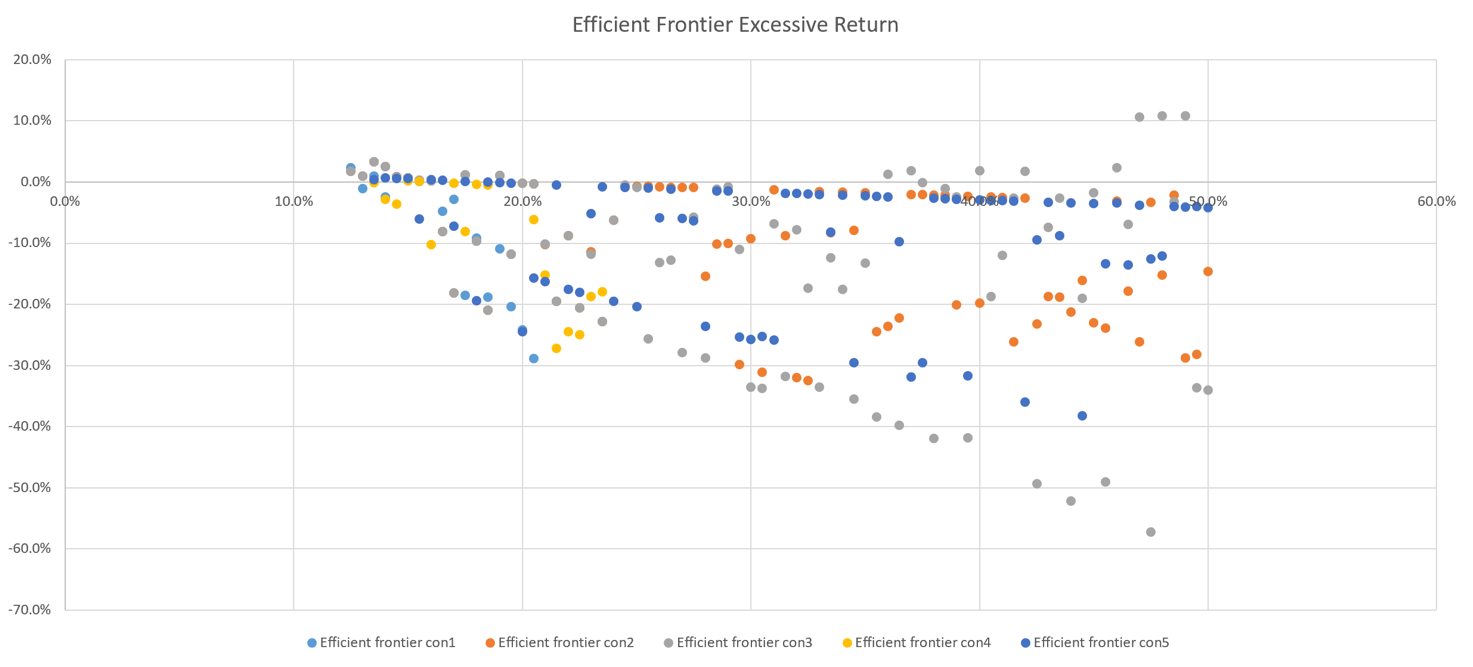
Figure 16: Excessive returns of efficient frontier.

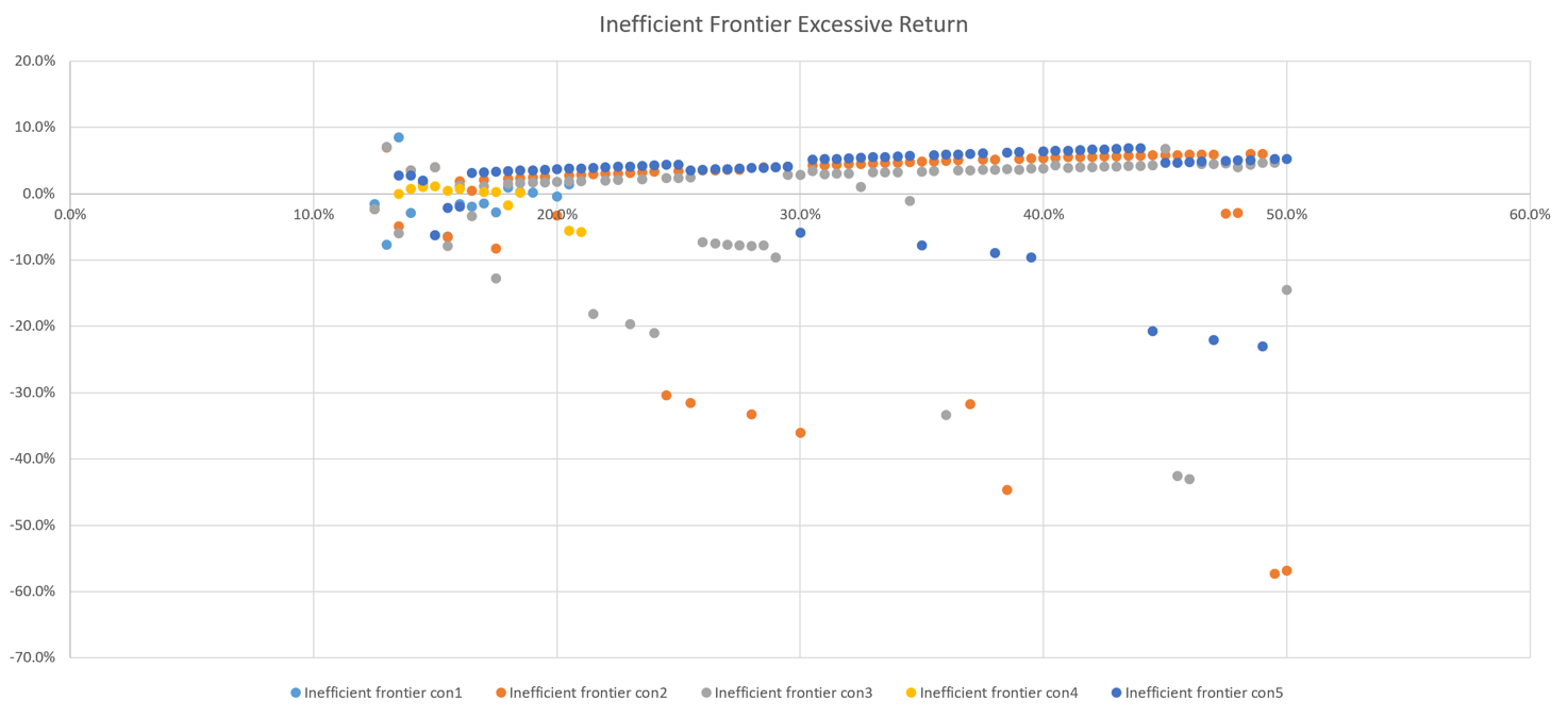
Figure 17: Excessive returns of inefficient frontier.

We found that the excessive return could be extremely high, especially when the target variance is high.

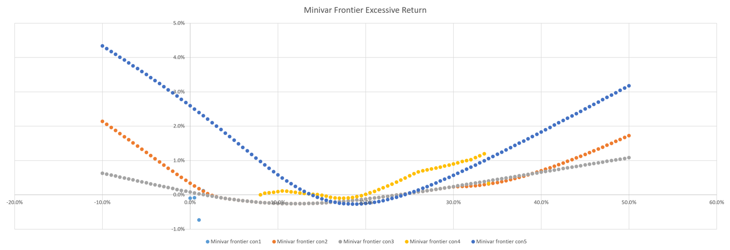
Figure 18: Excessive variance of minimum variance frontier.

For the Minivar Frontier, we calculated the excessive variance, and found that the variance of Markowitz Model is almost always higher than that of Index Model, which indicates that the Sharpe ratio estimated by Index Model is almost always higher. Also, we found that the excessive variance gets relatively higher when the target return is negative, one possible reason is that when the target return is negative, our portfolio tend to take a more radical strategy, causing the excessive variance to get higher.

As a result, since the excessive return can reach 56.9% in extreme situations, we can say that the robustness the two models is rather weak. However, with a target variance lower than 20%, the excessive return stays in a acceptable area, which means that the data could be reliable when the expected risk is low.

To assess robustness, we calculated the excessive return and excessive variance of the frontiers. Figures 16 to 18 illustrate that while the excessive return could be extremely high in certain scenarios, the excessive variance of the Markowitz Model was generally higher than that of the Index Model. This suggests that the Index Model may offer a higher Sharpe ratio under similar conditions.

In summary, the data processing phase meticulously prepared the dataset for robust comparison, ensuring the accuracy and reliability of our subsequent analysis. This comprehensive approach allowed for a thorough evaluation of the performance and applicability of the Markowitz and Index Models in portfolio management.

4. Conclusion

4.1. Research Conclusion

This paper provides a comprehensive analysis of the Markowitz Model and the Index Model in the context of portfolio management. Through theoretical examination and empirical evaluation, the study highlights the strengths and limitations of each model. The Markowitz Model, with its robust mathematical foundation, offers precise portfolio optimization by considering the covariance matrix of asset returns. However, its practical application is often hindered by the need for extensive data and computational intensity. On the other hand, the Index Model, with its simplified approach and reliance on market index data, provides a more accessible and less computationally demanding alternative. Despite its ease of use, the Index Model's assumptions about market efficiency and linearity of returns may not hold in all market conditions, leading to potential inefficiencies.

The empirical results demonstrate that the Markowitz Model tends to offer higher expected returns and Sharpe ratios, albeit with similar standard deviations to the Index Model. The study also reveals that under certain constraints, the differences between the two models become significant, impacting the portfolio's performance. The analysis of the efficient, inefficient, and minimum variance frontiers further underscores the importance of model selection based on specific investment objectives and market conditions.

4.2. Future Plan

Building on the findings of this paper, future research will focus on several key areas to enhance the applicability and efficiency of portfolio optimization models. First, the integration of modern computational techniques such as machine learning algorithms and big data analytics will be explored to improve the accuracy and efficiency of both the Markowitz and Index Models. By leveraging these advanced technologies, it will be possible to handle larger datasets and more complex market dynamics, thus providing more robust portfolio optimization solutions [11].

Second, the study will expand to include a broader range of asset classes and market conditions to assess the models' performance across different economic scenarios. This will provide a more comprehensive understanding of the models' strengths and weaknesses in diverse market environments.

Third, the development of hybrid models that combine the strengths of the Markowitz and Index Models will be investigated. Such models aim to offer a balanced approach that capitalizes on the precision of the Markowitz Model and the practicality of the Index Model, potentially leading to more optimal portfolio management strategies.

Lastly, future research will also explore the impact of behavioral finance on portfolio optimization. By incorporating behavioral factors into the models, it will be possible to account for irrational investor behaviors and market anomalies, leading to more realistic and effective portfolio strategies.

In conclusion, this study lays the groundwork for further advancements in portfolio optimization, paving the way for more sophisticated and practical investment strategies in an ever-evolving financial landscape.

References

[1]. Beste, A., Leventhal, D., Williams, J., & Lu, Q. (2002). The Markowitz Model. Selecting an Efficient Investment Portfolio”. Lafayette College, Mathematics REU Program.
[2]. Mangram, M. E. (2013). A simplified perspective of the Markowitz portfolio theory. Global journal of business research, 7(1), 59-70.
[3]. Sarker, M. R. (2013). Markowitz portfolio model: evidence from Dhaka Stock Exchange in Bangladesh. International Organization of Scientific Research Journal of Business and Management, 8(6).
[4]. Stone, B. K. (1974). Systematic interest-rate risk in a two-index model of returns. Journal of financial and quantitative analysis, 9(5), 709-721.
[5]. Hristache, M., Juditsky, A., & Spokoiny, V. (2001). Direct estimation of the index coefficient in a single-index model. Annals of Statistics, 595-623.
[6]. Al-Naif, K. L. (2017). The relationship between interest rate and stock market index: Empirical evidence from Arabian countries. Research journal of finance and accounting, 8(4), 181-191.
[7]. Alquier, P., & Biau, G. (2013). Sparse single-index model. Journal of Machine Learning Research, 14(1).
[8]. Kamil, A. A., Fei, C. Y., & Kok, L. K. (2006). Portfolio analysis based on Markowitz model. Journal of Statistics and Management Systems, 9(3), 519-536.
[9]. Naik, P. A., & Tsai, C. L. (2001). Single‐index model selections. Biometrika, 88(3), 821-832.
[10]. Best, M. J., & Hlouskova, J. (2000). The efficient frontier for bounded assets. Mathematical methods of operations research, 52, 195-212.
[11]. Pandey, M. (2012). Application of markowitz model in analyzing risk and return (a case study of bse stock). Ahmedabad Chief Editor, 43(1), 1-14.
Cite this article
Wu,E. (2024). Comparative Analysis on the Application of Markowitz Model and Index Model in Portfolios. Advances in Economics, Management and Political Sciences,94,187-201.
Data availability
The datasets used and/or analyzed during the current study will be available from the authors upon reasonable request.
Disclaimer/Publisher's Note
The statements, opinions and data contained in all publications are solely those of the individual author(s) and contributor(s) and not of EWA Publishing and/or the editor(s). EWA Publishing and/or the editor(s) disclaim responsibility for any injury to people or property resulting from any ideas, methods, instructions or products referred to in the content.
About volume
Volume title: Proceedings of ICFTBA 2024 Workshop: Finance in the Age of Environmental Risks and Sustainability
© 2024 by the author(s). Licensee EWA Publishing, Oxford, UK. This article is an open access article distributed under the terms and
conditions of the Creative Commons Attribution (CC BY) license. Authors who
publish this series agree to the following terms:
1. Authors retain copyright and grant the series right of first publication with the work simultaneously licensed under a Creative Commons
Attribution License that allows others to share the work with an acknowledgment of the work's authorship and initial publication in this
series.
2. Authors are able to enter into separate, additional contractual arrangements for the non-exclusive distribution of the series's published
version of the work (e.g., post it to an institutional repository or publish it in a book), with an acknowledgment of its initial
publication in this series.
3. Authors are permitted and encouraged to post their work online (e.g., in institutional repositories or on their website) prior to and
during the submission process, as it can lead to productive exchanges, as well as earlier and greater citation of published work (See
Open access policy for details).