1. Introduction

In California, paid sick leave, sometimes referred to as paid sick time or PSL requirements, is a long-term legislation that was put into place with the goal of enhancing employee wellbeing. To be more precise, PSL could be used to help workers—part-time, full-time, and temporary workers—who meet certain requirements heal from physical or mental illnesses, see a doctor, receive treatment, or take care of a family member who needs preventative care—all without endangering their job. [1]. It is required that employees in California stay for the same company for a minimum of thirty days in a year and finish a ninety-day work cycle before taking any paid sick leave. In California, the Healthy Workplaces, Healthy Families Act of 2014 came into effect on July 1, 2015, designed to address public health concerns and promote job security and economic stability for workers. However, the impacts of this mandate are far more than the superficial benefits, influencing various aspects of labor dynamics such as employment rates, labor force participation rate, absenteeism, labor productivity, and the overall health condition of the workforce. This study mainly focuses on the real-world effect of this mandate on the working hours of selected types of workers – full-time employees – in California state in the US.

In the developed world, the United States is one of the few OECD countries without a law requiring paid sick leave. On August 5 of the same year, 1993, President Bill Clinton signed the Family and Medical Leave Act (FMLA) into law [2]. Allowing staff members to take suitable unpaid leave as a result of a serious sickness, an ailing family member, or a sick kid helps them manage their professional and personal responsibilities. Although FMLA was the first federal law to protect workers in similar circumstances, unpaid leave is still a significant flaw of it. Workers must have worked for their employers for a minimum of 12 months and 1,250 hours in the prior year in order to be eligible for FMLA benefits. Furthermore, the company needs to employ fifty or more people. In addition, some claim that the majority of workers receiving FMLA benefits are middle-class and upper-class workers. This is because, as opposed to workers with low incomes, they are more likely to receive paid time off options from their employers. Additionally, companies in the private sector are not required to provide paid sick leave to their employees. As a result, it is estimated that 44% of US employees do not have access to FMLA leave [3].

Introducing the PSL mandate led to a modest increase in employment rates [4]. This is attributed to the reduction in working while sick, which improves overall productivity and the healthy condition of workers, leading to job retention and a reduced level of turnover. Besides, Employers adjust to PSL mandates without substantial layoffs or reductions in workforce size. The mandates encourage a healthier work environment, which will enhance worker satisfaction and productivity.

As a result, employees without having PSL may go to work while sick. This could not only prolong illness but also lead to workers being less productive than those in healthy conditions [5]. With sick workers in the office, contagious diseases and illnesses are highly likely to spread throughout the workplace. According to the research by Smith, around 68% percent of employees suffer from stomach flu or contagious diseases while working at the workplace [6]. Moreover, without PSL, workers may face a trade-off between recovering at home without pay and earning to work. Mostly, the more severe the illness, the more recommended that employees should stay at home for recuperation. For many workers, the opportunity cost of staying at home exceeds that of going to work; hence, they will continue working while suffering from illness [7]. That is to say, the introduction of Paid Sick Leave could not only assist the sick people themselves to recover soon but also benefit the colleagues around them by not being affected by those infectious diseases. It is possible that the PSL could reduce and mitigate sick leave, as well as the spread of disease [8].

Under such considerations, eleven states and one federal district passed PSL mandates, as shown in Table 1. Even though some detailed rules may vary between different regions, the majority of the mandates are similar.

Table 1: Published Year of Paid Sick Time Laws in different states

For every thirty hours worked, employees in California who are subject to the PSL obligation will be given one hour of paid leave. The total amount of paid sick leave that an employee may accrue is restricted by the employer to either 80 hours or 10 days or 40 hours or 5 days annually. Employers are not required to allow workers to use more than forty hours (or five days) of paid leave yearly, and carryover is not required if the whole authorized time is utilized at the very beginning of the leave year. However, employees are allowed to carry over any unused paid sick leave.

The reason for using full-time workers in this research is that the impact of the mandate on full-time employees may be greater than that on part-time employees. Due to the differences in the nature of work between full-time and part-time employees, full-time roles typically require a set number of hours per week (e.g., 40 hours). That is to say, paid sick leave allows full-time employees to miss work without financial penalty, temporarily reducing their working hours. In contrast, part-time roles are often more flexible with fewer guaranteed hours and may already have varying schedules; thus, a significant change might not be observed in their overall working hours due to paid sick leave. In other words, after PSL existed, part-time employees may see less change in their working hours, whilst there could be a more evident impact on full-time workers. Therefore, this study mainly focuses on the impact of the PSL on the labor dynamics of part-time employees.

2. Methodology

In this study, the impact of the publication of PSL in 2015 in California state on full-time employees’ weekly working hours is expected to be investigated. The Diff-in-Diff (DiD) model is a quasi-experimental method. When randomization of treatment assignment is impractical, econometricians and social scientists utilize the DiD model, a statistical tool, to estimate the causal influence of a treatment or intervention. It contrasts how a group receiving a policy change (the treatment group) and a group not receiving that (the control group) evolve over time in terms of outcomes.

The underlying premise of the DiD approach is the parallel trends assumption, which asserts that the treatment and control groups' result patterns would have eventually followed a similar pattern in the absence of the shock [9]. Apart from that, another two assumptions are: the introduction of treatment does not affect the control group’s outcomes, and there are no anticipations.

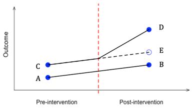
Figure 1: Difference-in-Difference (DiD) Model

Photo credit: Originals

When evaluating a policy change, cross-section estimator can be used to compare treated to control observations at one point in time, while the omitted variable bias could arise, even when including additional covariates. Another estimator – before-after estimator – compares treated observations after the policy change to treated observations before the policy change, but it may estimate a time-trend that would have happened even without the policy change. Using the concepts of the above two estimators, DiD estimator can be set up in two ways. Firstly, using the difference between before-after difference for treated ( \( y_D - y_C \) ) and before-after difference for controls ( \( y_B - y_A \) ), as the latter difference can be approximated for the time trend for treated group ( \( y_E - y_C \) ) would have been without the policy change. Second way is using the difference between cross-section difference for treated and control in post ( \( y_D - y_B \) ) and pre period ( \( y_C - y_A \) ). In this scenario, the difference in the pre period could be used as a proxy for what the difference between treated and control would have been had it not been for the policy change.

2.1. Source of data

Data from the Current Population Survey (CPS) are used in this article. It is the United States Census Bureau's monthly household survey on employment and labor markets, which was carried out in March for the Bureau of Labor Statistics. The extracts include individual data for about 150,000 individuals each year who are selected by a multistage stratified statistical sampling scheme. It offers detailed demographic and labor force data on the civilian non-institutionalized population aged 16 and older in the US. The survey covers a broad spectrum of topics, including employment status, hours worked, wages, industry, education, and core demographic variables: age, sex, race, ethnicity, etc.

2.2. Model Specification

Within the model, full-time employees in California state are selected to be the treatment group, and the full-time workers in Texas state are assigned to be the control group. According to Table 1, both the California and Massachusetts governments published PSL in 2015 compared to others. Thereafter, the year 2011 became a crucial point in time, which is the primary turning point. The research focuses on how the time trends in the weekly working hours within the treatment and control groups changed from 2014 to 2015 and from 2015 to 2016, investigating the impact of the publication of PSL. If a notable difference is observed within that time period, it would provide a supportive argument for the research.

In addition, a multiple linear regression method is used to provide a more statistically robust analysis. The model is:

\[ uhours=\beta_0+\beta_1·treat+β_{2}·post+β_{3}·treat∗post+β_{i}·controls+γ_{t}+ϵ \] (1)

Where:

• uhours is the average weekly working hours for the employees in California and Texas.

• treat is a dummy variable, where it assigns treat = 1 for treatment group (employees in California), treat = 0 for control group (employees in Texas).

• post is a dummy variable which when post = 1 represents time after 2015, while post = 0 for time before 2015.

• treat * post is an interaction term between variables treat and post.

• controls represents control variables that may have effect on dependent variable.

\( \beta_0 \) indicates the intercept, and \( \beta_1 \) to \( \beta_i \) the estimated coefficients for the independent variables.

\( \gamma _t\ \) shows the time fixed effects.

\( \epsilon \) represents the residuals.

2.3. Descriptive Statistics

The CPS data used in this research paper is from 2011 to 2019 and covers the years before and after the policy was implemented. Two states: California and Texas states are selected, where the treatment group is California state and the other state is the control group. The reason why Texas was chosen to examine how PSL affected the working hours of full-time employees are listed as follows.

Table 2: Summary Statistics for California State

From the two tables (Table 2 and Table 3, the summary statistics of 5 control variables of full-time employees in both states are shown. The average age in both states was around 40, with a similar standard deviation of about 13.6. Besides, those workers in both states have similar years of education. When it comes to the two dummy variables: sex and marital status, both mean and standard deviation in the two states are almost the same. There is only a minor difference observed in the hourly wage variable, but it does not affect the outcome of the analysis substantially. Above all, with the high similarity of most of the standard deviation and mean of control variables of the two states, the time trend for the treated group can be guaranteed.

Table 3: Summary Statistics for Texas State

3. Results

3.1. Line Plot Result

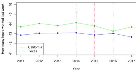
Figure 2 illustrates the weekly working hours over time in California and Texas state. On the horizontal axis are the years, while the weekly working hours of full-time employees in both states over the years are on the vertical axis. The Blue line indicates the treatment group – California state, and the green line represents the control group – Texas state.

Figure 2: California – Texas

Photo credit: Original

Prior to the publication of the mandate in July 2015 in California state, the time trends of full-time employees’ weekly working hours within both states appeared to be flat with similar fluctuations. However, after 2015, a notable divergence is observed between the two states, coinciding with the publication of PSL. While the weekly working hours in Texas state kept decreasing, which is perceived as a consistent trend, a rise in the weekly working hours of full-time employees in California is observed.

Therefore, two expectations on the result from the regression models are formed. First and foremost, a positive value of the DiD estimator should be expected – which is the interaction term. Secondly, the estimator should be statistically significant; that is, \( \beta_3 \) should be at least at 5% level of significance.

3.2. Regression Model Result

As can be seen in Table 4, two regression models are used. Both regression models add fixed year effects to address the potential issue of weekly working hours variations over time.

Table 4: Regression Model Result

(1): The link between the treatment variable, post-treatment periods, and the interaction term between treat and post are examined in the baseline regression.

(2): This regression model is based on the model (1), by introducing control variables into the regression. Hence, the determinants of working hours of full-time employees can be analyzed. For example, controlling education, marital status, sex, age, age squared could give a better explanation on the impact of treatment variable on weekly working hours while holding other factors constant.

Overall, the estimated coefficient of treat * post-term ( \( \beta_3 \) ) in both models is statistically significant at a 5% significant level, which means that our findings are robust. Secondly, the introduction of control variables does not bring about a significant change in the estimated coefficients so omitted variable bias can be ignored. When looking at the coefficient of interaction term itself, around 0.76, it shows that holding all other factors constant, the introduction of the Paid Sick Leave mandate in California state in 2015 caused full-time employees’ weekly working hours to increase by around 0.76 hours on average. Due to the fact that the act was in effect in July 2015, and the data were collected in March 2016, the time lag between the implementation and real-world effect can be neglected. That is to say, the publication of PSL in 2015 has positively affected the weekly working hours of employees in California state [10].

4. Conclusion

To conclude, the study provides strong evidence that the PSL in California State gave rise to a positive impact on the labor dynamic, and the weekly working hours of full-time employees. Using the Difference in Difference (DiD) approach and Current Population Survey data, a clear difference between weekly working hours between Texas state and California state is observed, which is then confirmed statistically significantly by the regression model. The positive direct effect of PSL on weekly working hours may be caused by a reduction in the duration of illness as staying at home for recovery may not be time-consuming. Furthermore, the PSL could even improve working hours by enhancing public health conditions so that the probability of catching the flu or being sick is decreased. Especially in the service industry, sick workers are likely to spread disease to their customers, causing ripple effects.

However, due to the data availability, the study cannot evaluate the reasons behind leaving. For example, workers may accumulate PSL in the first year (2016), and use up two-year paid leave in the second year for purposes other than sick leave. Also, even though the time lag of implementation of the PSL can be neglected, workers who receive this mandate may not respond positively fearing that it will bring about adverse effects on the employer’s impression of them. Thus, everyone is waiting for the first worker to use PSL.

Lastly, this study contributes to bridging a gap in the related research areas, by considering full-time employees instead of the entire population, which could assist policymakers or employers to contribute to a better labor market.

References

[1]. Paid Sick Leave in California. (n.d.). Www.dir.ca.gov. https://www.dir.ca.gov/dlse/California-Paid-Sick-Leave.html
[2]. U.S. Department of Labor. (2022). FMLA (Family & Medical Leave). U.S. Department of Labor. https://www.dol.gov/general/topic/benefits-leave/fmla
[3]. Golden, R. (2023, February 3). FMLA: The 30-year legacy of a celebrated — and complicated — employment law. HR Dive. https://www.hrdive.com/news/fmla-30th-anniversary-history-paid-leave/641972/
[4]. Pichler, S., & Ziebarth, N. R. (2020). Labor market effects of US sick pay mandates. Journal of Human Resources, 55(2), 611-659.
[5]. Earle, A., & Heymann, J. (2020). A comparative analysis of paid leave for the health needs of workers and their families around the world. In Policy Sectors in Comparative Policy Analysis Studies (pp. 150-166). Routledge.
[6]. Heymann, J., Rho, H. J., Schmitt, J., & Earle, A. (2010). Ensuring a healthy and productive workforce: comparing the generosity of paid sick day and sick leave policies in 22 countries. International Journal of Health Services, 40(1), 1-22.
[7]. Stearns, J., & White, C. (2018). Can paid sick leave mandates reduce leave-taking?. Labour Economics, 51, 227-246.
[8]. Li, J., Birkhead, G.S., Birkhead, G.S., Strogatz, D.S., Coles, F.B., & Coles, F.B. (1996). Impact of institution size, staffing patterns, and infection control practices on communicable disease outbreaks in New York State nursing homes. American journal of epidemiology, 143 10, 1042-9.
[9]. Ryan, A. M., Kontopantelis, E., Linden, A., & Burgess Jr, J. F. (2019). Now trending: Coping with non-parallel trends in difference-in-differences analysis. Statistical methods in medical research, 28(12), 3697-3711.
[10]. Callison, K., & Pesko, M. F. (2022). The effect of paid sick leave mandates on coverage, work absences, and presenteeism. Journal of Human Resources, 57(4), 1178-1208.
Cite this article
Xia,N. (2024). Paid Sick Leave Mandate and Its Impact on Labor Dynamics in California. Advances in Economics, Management and Political Sciences,103,62-69.
Data availability
The datasets used and/or analyzed during the current study will be available from the authors upon reasonable request.
Disclaimer/Publisher's Note
The statements, opinions and data contained in all publications are solely those of the individual author(s) and contributor(s) and not of EWA Publishing and/or the editor(s). EWA Publishing and/or the editor(s) disclaim responsibility for any injury to people or property resulting from any ideas, methods, instructions or products referred to in the content.
About volume
Volume title: Proceedings of the 8th International Conference on Economic Management and Green Development
© 2024 by the author(s). Licensee EWA Publishing, Oxford, UK. This article is an open access article distributed under the terms and
conditions of the Creative Commons Attribution (CC BY) license. Authors who
publish this series agree to the following terms:
1. Authors retain copyright and grant the series right of first publication with the work simultaneously licensed under a Creative Commons
Attribution License that allows others to share the work with an acknowledgment of the work's authorship and initial publication in this
series.
2. Authors are able to enter into separate, additional contractual arrangements for the non-exclusive distribution of the series's published
version of the work (e.g., post it to an institutional repository or publish it in a book), with an acknowledgment of its initial
publication in this series.
3. Authors are permitted and encouraged to post their work online (e.g., in institutional repositories or on their website) prior to and
during the submission process, as it can lead to productive exchanges, as well as earlier and greater citation of published work (See
Open access policy for details).