1. Introduction

Stock market return forecasting has been one of the core issues in the field of finance, while it is closely related to other finance issues such as portfolio management, cost of funds, and market effectiveness. At present, numerous studies have found that there is a nonlinear correlation beyond the classical linear correlation in stock market returns, which does not satisfy the assumption of random wandering, and that there is a predictable component behind the complex surface of stock price fluctuations.

From the efficient market hypothesis to Markowitz mean-variance theory and from Tobin's two-fund separation theorem to the Capital Asset Pricing Model (CAPM) proposed by Sharpe et al. in the early 1960s, the quest for modern investment theory shifted from normative theory to empirical research. The CAPM model makes the assumption that systematic risk alone determines expected stock returns. However, subsequent research has demonstrated that many more underlying factors, such as the three-factor model proposed by Fama and French[1] and the improved five-factor model proposed by Fama and French[2], explain asset returns. In these models, the factor returns are typically estimated using cross-sectional regressions. Each factor in an asset pricing framework can be represented as a portfolio whose returns are the same as the factor's returns.

Deep learning is all about predicting asset returns by finding non-linear factors, and thus the predictability of stock returns can be studied using multilayer deep learning models. Combining deep learning with layered nonlinear factors for out-of-sample prediction provides an alternative to dynamic factor modeling.

By classifying stocks by style, nation, or industry, LSTM models are an effective tool for predicting returns and assisting portfolio managers and investors in making investment decisions. To project stock market returns throughout several forecast windows, Mojtaba Nabipour, Pooyan Nayyeri, Hamed Jabani, and Amir Mosavi[3] compare the results of various deep learning models and other machine learning techniques. They employ Decision Tree, Bagging, Random Forest, Adaptive Boosting (AdaBoost), Gradient Boosting and eXtreme Gradient Boosting (XGBoost), Artificial neural network (ANN), Recurrent Neural Network (RNN), and Long short-term memory (LSTM), where ANN, RNN, LSTM belong to neural networks. When using various regression loss measures, LSTM outperforms the other algorithms in terms of accuracy and model-fitting ability. From 1992 until 2015, LSTM networks were used by Fischer and Kraus[4] to forecast out-of-sample directional movements for the stocks that make up the S&P 500. They discovered that LSTM networks perform better than memory-free classification techniques like logistic regression classifiers (LOG), deep neural nets (DNN), and random forests (RAF).

To assist investors in obtaining higher excess returns, I use long short-term memory (LSTM) to perform an empirical investigation on the predictability of stock market returns in this paper.

2. Methodology

2.1. Artificial Neural Network

2.1.1. RNN

Both temporal and semantic information can be mined by the recurrent neural network, which performs incredibly well on data having sequential features. It is able to recall information about each moment, and the hidden layer at each moment is controlled not only by the input layer at that moment but also by the hidden layer from the previous moment. Deep learning models have made significant progress in addressing issues in natural language processing (NLP) domains such speech recognition, language modeling, machine translation, and temporal analysis thanks to the utilization of recurrent neural networks' capability.

A simple recurrent neural network is composed of an input layer, a hidden layer, and an output layer. [5] U is the weight matrix from the input layer to the hidden layer; O is a vector that represents the output layer's values; V is the weight matrix from the hidden layer to the output layer; and the weight matrix W is the weight of the hidden layer's final value as an input. After receiving the input at moment t, the value of the hidden layer is and the output value is. The calculation of a recurrent neural network can be represented by the following equation:

\( {O_{t}}= \) g (V · \( {S_{t}} \) ) (1)

\( {S_{t}}= \) f (U · \( {X_{t}}+ \) W · \( {S_{t-1}} \) ) (2)

Since RNN suffers from gradient vanishing[6] problems during backpropagation, it is difficult to handle remote dependency. Therefore, a series of related variants have been generated from it, such as LSTM and GRU[7].

2.1.2. LSTM

LSTM[8] is a form of RNN that has numerous applications, including time series analysis, document categorization, speech and voice recognition. While the basic version of RNN stores all information, LSTM stores information selectively, using a gate to control each moment of information remembering and forgetting, which can solve the gradient vanishing or exploding problem in RNN.

A forgetting gate[9] selectively forgets some components that were in the previous cell state. The forgetting gate's computation can be described using the equation below, where \( {f_{t}} \) is the output vector of the sigmoid neural layer:

\( {f_{t}}= \) σ ( \( {W_{f}} \) · [ \( {h_{t-1}}, {x_{t}} \) ] + \( {b_{f}} \) ) (3)

The memory gate determines whether the data at instant t is merged into the unit state. The system extracts valid information from the input and filters it, assigning a rating (0 ~ 1) to each component. The higher the rating, the more memory is incorporated into the unit state. The following equation can be used to describe the computation of the memory gate:

\( {C \prime \prime _{t}}= \) tanh ( \( {W_{c}} \) · [ \( {h_{t}}- 1 \) ] + \( {b_{c}} \) ) (4)

\( {i_{t}}= \) σ ( \( {W_{i}} \) · [ \( {h_{t-1}}, {x_{t}} \) ] + \( {b_{i}} \) ) (5)

Finally, the output layer will integrate the vector of the current input values with the output values of the previous moment to extract the information in it using the sigmoid function, and then compressively map the current state of the unit into the interval (-1, 1) by the tanh function.

2.2. Test Methods

2.2.1. In-sample testing

The usual regression model[10] for conventional yield forecasts is:

\( {r_{t}}= \) α + β \( {x_{t-1}} \) + \( {ε_{r, t}} \) (6)

\( {r_{t}} \) represents the excess return; \( {x_{t-1}} \) represents the predictor; α represents the intercept term; β represents the coefficient of influence of the predictor on the return, and if β = 0, the factor is not predictive of the return; ε is the residual term. However, Lewellen J. has shown that the direct estimation is biased. Therefore, the FQGLS method propose by Westerlund and Narayan[11] is used to overcome the problems of persistence, heteroskedasticity and endogeneity of the data itself. The t-statistic can be expressed as:

\( {t_{FQGLS}}=\frac{\sum _{t={q_{m+2}}}^{T}π_{t}^{2}x_{t-1}^{d}r_{t}^{d}}{\sqrt[]{\sum _{t={q_{m+2}}}^{T}Π_{t}^{2}{(x_{t-1}^{d})^{2}}}} \) (7)

\( x_{t}^{d} \) = \( {x_{t}} - \sum _{s=2}^{T}\frac{{x_{s}}}{T} \) (8)

\( r_{t}^{d} \) = \( {r_{t}} - \sum _{s=2}^{T}\frac{{r_{t}}}{T} \) （9)

\( {π_{t}} \) = \( \frac{1}{{σ_{ηt}}} \) (10)

2.2.2. Out-of-sample testing

Based on Rapach D E, Strauss J K, Zhou G.[12][13], assuming a total sample length of 2t periods, the entire sample is divided into an estimation sample (the first t periods) and a prediction sample (the last t periods). The model parameters are estimated using the least squares method for the first t-period estimation sample, and then the returns for the t+1-period are predicted, iterating until the entire prediction sample is calculated. Finally, the empirical results are analyzed using relative mean absolute error, relative root mean square error, and out-of-sample \( {R^{2}} \) as indicators of out-of-sample predictive effectiveness.

Relative Mean Absolute Error (RMAE) can be computed using the formula below:

\( RMAE=\frac{\sum _{t+1}^{2t}\frac{|{r_{i}}- {rˆ_{i}}|}{t}}{\sum _{t+1}^{2t}\frac{|{r_{i}}- {r̄_{i}}|}{t}} \) (11)

Relative Root Mean Square Error (RRMSE) can be computed using the formula below:

\( RRMSE=\frac{\sqrt[]{\sum _{t+1}^{2t}\frac{|{r_{i}}- {rˆ_{i}}|}{t}}}{\sqrt[]{\sum _{t+1}^{2t}\frac{|{r_{i}}- {r̄_{i}}|}{t}}} \) (12)

Out-of-sample variance ( \( {OR^{2}} \) ) can be computed using the formula below:

\( {OR^{2}}=1- \frac{\sum _{t+1}^{2t}{({r_{i}}- {rˆ_{i}})^{2}}}{\sum _{t+1}^{2t}{({r_{i}}- {\bar{r}_{i}})^{2}}} \) (13)

When RMAE and RRMSE are less than 1 and \( {OR^{2}} \) is more than 0, it indicates that the selected component outperforms the historical mean model in terms of predicting ability and out-of-sample.

2.3. Data

2.3.1. Data collection

Monthly data of S&P500 index for the years 1871-2019 are selected as stock market returns in this paper. The log dividend price ratio; log earnings price ratio; volatility; three-month Treasury bill yields; ten-year Treasury bill yields; term spreads (the gap between the yields on ten-year Treasury bills and three-month Treasury bills); credit spreads (the gap between the yields on AAA-rated corporate bonds and ten-year Treasury bills); inflation (PPI Producer Price Index inflation); the growth rate of industrial production; M(1,12) (the S&P500 price index is greater than or equal to its 12-month moving average, which takes the value of 1; if less, it takes the value of 0); M(3,12) (the three-month moving average of the S&P500 price index is greater than or equal to its 12-month moving average, which takes the value of 1; if less, it takes the value of 0); and MOM(6) (if the S&P500 price is more than or equal to the value of the S&P500 price 6 months ago, MOM(6) takes the value of 1; if less, it takes the value of 0) are the twelve indicators[14] used as predictor variables for the return predictability study.

2.3.2. Data analysis

The data is screened and processed to obtain a suitable data set. Plotting a time series of features can help identify trends, seasonal and cyclical variations. Figure 1 shows the twelve variables used in this experiment.

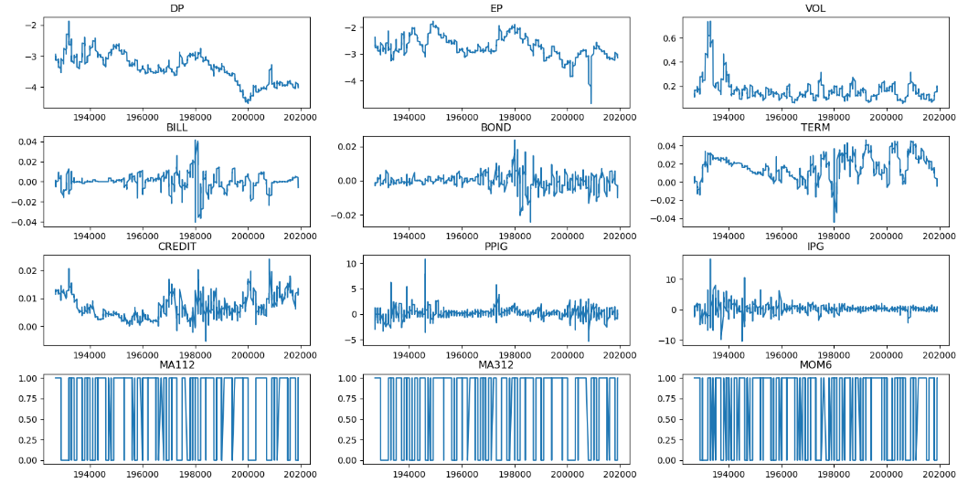
Figure 1: Visualisation of twelve variables.

Visualize the correlation between features by calculating the correlation matrix between features and plotting a correlation heat map (see Figure 2). From the correlation matrix, it can be seen that there is a strong correlation between some of the predictors while others have little to no correlation.

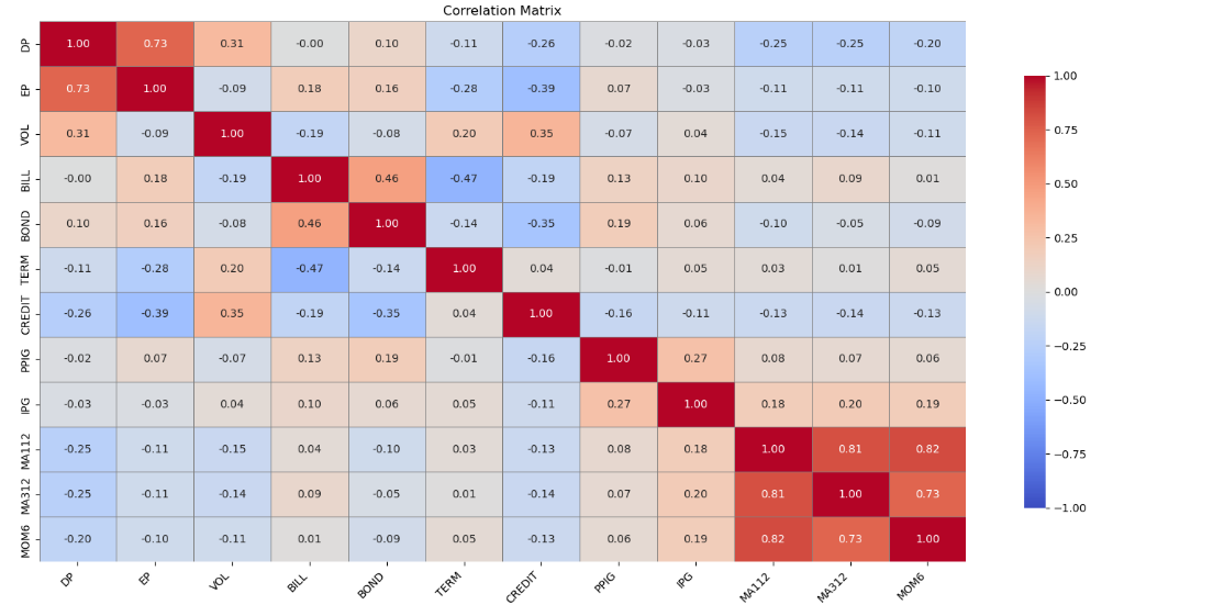
Figure 2: Heat map of correlations for each variable.

The variables DP and EP are highly positively correlated, indicating that the Dividend Price Ratio and the Earnings Price Ratio have historically shown similar trends. There is a strong positive correlation between the three technical indicators MA112, MA312 and MOM6, probably because they are all calculated based on moving averages of prices, reflecting similar market trends. The positive correlation between VOL and CREDIT suggests that there is a relationship between market volatility and credit spreads, possibly reflecting the fact that credit spreads widen when market volatility is high. The negative correlation between VOL and TERM suggests that term spreads may narrow when market volatility is high.

Strong correlations may mean that these variables provide less independent information in the model, while low correlations may provide more independent information. It helps to understand the role of individual predictors and informs further model construction and optimization.

Then, we train the model using training data and evaluate it on a validation set. Last, use metrics such as RMSE, MAE, etc. to evaluate the predictive performance of the model.

3. Results

3.1. OLS

The out-of-sample test of the multifactor model was performed on the monthly data of the S&P500 index for the years 1871-2019 by using the data from December 1956 and before as the sample data for the training set and the data from December 1956 onwards as the sample data for the test set.

Out-of-sample tests were carried out on the multifactor model using the OLS approach. In the test of statistical gain, the results show an out-of-sample R² of -0.032711, which is a measure of the predictive performance of the model and usually takes values between 0 and 1. Negative values indicate that the model is a poor predictor, even worse than a simple mean prediction. Thus the model fits very poorly on out-of-sample data and the model fails to effectively capture the information in the out-of-sample data. The adjusted MSFE of 2.848436 reflects the error between the predicted and actual values, with larger values indicating larger errors. p-value of MSFE is 0.004513, which indicates that the model's prediction error is statistically significant at the 5% level of significance. Taken together, the model has no predictive power on out-of-sample data.

This may be because the model is overfitted on the training data and fails to generalize effectively to out-of-sample data, or the selected features are not effective in explaining the variation in the out-of-sample data.

In the test of economic gain, the delta utility of 0.000494 measures the improvement in economic returns from investments made through the predictive model, and a positive value indicates that the predictive model makes economic sense. a smaller value of delta utility indicates that the predictive model makes some economic sense, but that there is room for improvement.

3.2. LSTM

Stock market returns are predicted using an LSTM model with 80% of the data used as the training set in the model. Fixed length historical data is used and the time step is set to 12 to enable the model to capture the time dependence and trends in the data. Train the model using the training set and use 20% of the data as the validation set.

From the change of loss during the training process, it can be seen that the training loss and the validation loss are gradually decreasing and finally stabilizing. It represents that the model gradually learnt the patterns in the data during the training process. And the difference between the training loss and the validation loss is not large, indicating that there is no obvious overfitting phenomenon. The experimental results show that the final training loss is 0.0065, which indicates that the model has less error on the training data and can fit the training data better. The final test loss is 0.0053, which is similar to the value of the training loss, which indicates that the model performs more consistently on the training set and the test set, and has better generalization ability. Meanwhile, the RMSE of the training set is 0.0566, which indicates that the prediction error on the training data is small; the RMSE of the test set is 0.0511, which indicates that the model's prediction error on the test data is also small, which verifies the model's prediction ability. The MAE is 0.0398 for the training set and 0.0393 for the test set, which is a lower MAE, further indicating a smaller prediction error. To show the trend of training and validation loss more visually, it can be analyzed by plotting the loss curve (see Figure 3).

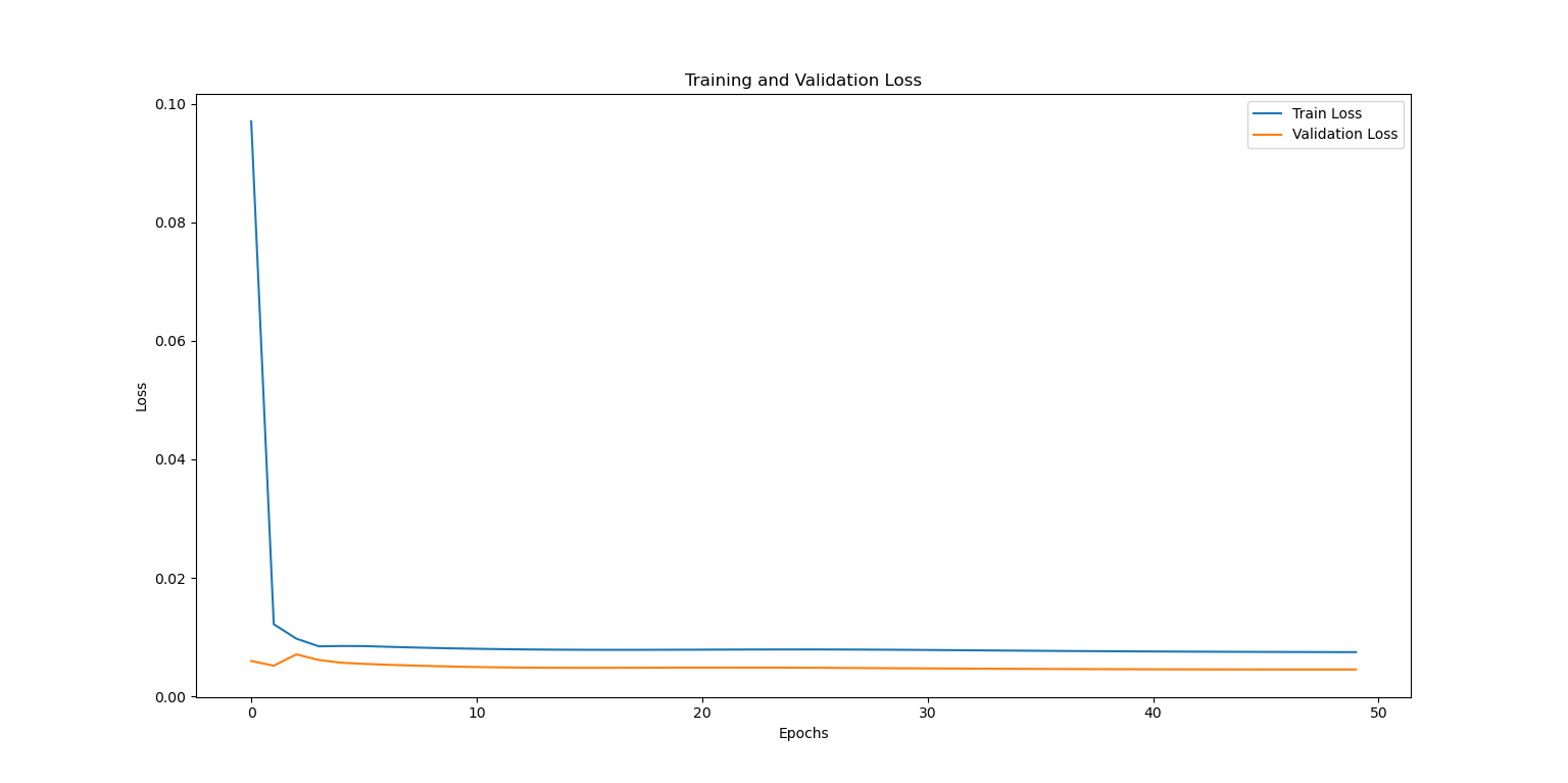
Figure 3: Visualisation of twelve variables.

A training set \( {R^{2}} \) of 0.0190 indicates that the model is a very poor fit to the training data. values of \( {R^{2}} \) range from 0 to 1, with values closer to 1 indicating that the model is better able to account for the variation in the data. an \( {R^{2}} \) of 0.0190 indicates that the model can only account for about 1.9% of the variation in the training data, which implies that the model captures little of the data's patterns and relationships in the training set. A test set R² of -0.5764 indicates that the model is very poor at predicting the test data. a negative \( {R^{2}} \) value means that the model is not even as good at predicting as it would be if it simply used the average of the data. This indicates that the model is severely overfitted and cannot generalize to new data. Therefore, the current features may not be sufficient to explain the variation in the target variable and more relevant features need to be introduced.

4. Discussion

A negative \( {R^{2}} \) value indicates that the model is not effectively explaining the variability of the data. The data may have problems such as noise, outliers or a weak relationship between the characteristics and the target variable. Afterwards, more features related to stock market returns can be introduced, such as technical indicators and macroeconomic indicators. Or correlation analysis or feature selection methods can be used to select features that have a significant impact on forecasting. Or the model parameters can be changed to try different model structures, such as increasing the number of LSTM layers or the number of neurons. Find the best time step that captures the time series patterns better by choosing different time steps. We can also try to integrate multiple models, such as LSTM with traditional time series models (ARIMA), Random Forest, XGBoost, etc., for integrated learning. The predictive performance and stability of the model can be further improved by introducing more features, optimizing the model structure, performing hyperparameter tuning and data processing.

5. Conclusion

Accurate forecasting of stock market returns is crucial for financial decision-making. Improved forecasting models can enhance investment strategies, optimize portfolio management and contribute to market stability. By evaluating traditional OLS models and advanced LSTM models using historical data of the S&P500 index (1871-2019), we aim to discover the predictive power of various financial metrics, contributing to the continuous search for better predictive tools in the financial sector, demonstrating the potential and challenges of deep learning methods.

The traditional OLS model shows a poor fit to out-of-sample data with an R² of -0.032711, indicating no predictive power. The adjusted MSFE value is 2.848436 with a statistically significant p-value of 0.004513, further confirming that the model is insufficient to predict stock returns. The economic return, measured by the delta effect, is slightly positive at 0.000494, indicating some economic significance, but the overall performance of the OLS model is unsatisfactory.

In contrast, the LSTM model, a more sophisticated deep learning approach, showed better agreement between training and validation losses, highlighting its generalizability. The LSTM model exhibited a consistent decline in training and validation losses, indicating its ability to learn from the data. However, the low training set R² (0.0190) and negative test set R² (-0.5764) revealed significant overfitting and a failure to generalize to unseen data. This suggests that while LSTM models can potentially capture intricate patterns in stock returns, they require further refinement to be practical and reliable.

Improved forecasting models can aid investors and portfolio managers in making informed decisions, potentially leading to higher returns and reduced risks. And policymakers can use enhanced predictive models to anticipate market movements, enabling more proactive and informed economic policies.

In the future, the explanatory power of the model can be improved by introducing more relevant features such as technical indicators and macroeconomic factors as well as sentiment analysis from news and social media. Model performance can be improved by experimenting with different LSTM architectures, as stacking multiple LSTM layers or integrating with other neural network types. Combining LSTM with other models such as ARIMA, Random Forest and XGBoost to capitalise on the strengths of each method and improve overall predictive accuracy and robustness. The development of models that are capable of dynamically updating and adapting in real-time, contingent upon the influx of data streams, holds considerable promise for informing pragmatic, day-to-day investment decisions.

References

[1]. Fama, E.F., & French, K.R. (1993). Common risk factors in the returns on stocks and bonds. Journal of Financial Economics, 33, 3-56.
[2]. Fama, E.F., & French, K.R. (2014). A Five-Factor Asset Pricing Model. S&P Global Market Intelligence Research Paper Series.
[3]. Nabipour, M., Nayyeri, P., Jabani, H., & Mosavi, A.H. (2020). Deep Learning for Stock Market Prediction. Entropy, 22.
[4]. Fischer, T.G., & Krauss, C. (2017). Deep learning with long short-term memory networks for financial market predictions. Eur. J. Oper. Res., 270, 654-669.
[5]. Zaremba, W., Sutskever, I., & Vinyals, O. (2014). Recurrent Neural Network Regularization.
[6]. Tan, H.H., & Lim, K. (2019). Vanishing Gradient Mitigation with Deep Learning Neural Network Optimization. 2019 7th International Conference on Smart Computing & Communications (ICSCC), 1-4.
[7]. Bengio, Y., Simard, P.Y., & Frasconi, P. (1994). Learning long-term dependencies with gradient descent is difficult. IEEE transactions on neural networks, 5 2, 157-66 .
[8]. Hochreiter, S. , & Schmidhuber, J. . (1997). Long short-term memory. Neural Computation, 9(8), 1735-1780.
[9]. Deutsch. (2012). Supervised sequence labelling with recurrent neural networks | springer. Springer-Verlag Berlin Heidelberg.
[10]. Montgomery, D.C., & Peck, E.A. (2001). Introduction to Linear Regression Analysis.
[11]. Westerlund, J., & Narayan, P.K. (2015). Testing for Predictability in Conditionally Heteroskedastic Stock Returns. Journal of Financial Econometrics, 13, 342-375.
[12]. Rapach, D.E., Strauss, J., & Zhou, G. (2009). Out-of-Sample Equity Premium Prediction: Combination Forecasts and Links to the Real Economy. Capital Markets: Asset Pricing & Valuation eJournal.
[13]. Rapach, D.E., & Wohar, M.E. (2006). In-sample vs. out-of-sample tests of stock return predictability in the context of data mining. Journal of Empirical Finance, 13, 231-247.
[14]. Rapach, D.E., & Zhou, G. (2019). Time-Series and Cross-Sectional Stock Return Forecasting: New Machine Learning Methods. ERN: Other Econometric Modeling: Capital Markets - Forecasting (Topic).
Cite this article
Yu,S. (2024). Advancing Stock Market Return Forecasting with LSTM Models and Financial Indicators. Advances in Economics, Management and Political Sciences,122,137-144.
Data availability
The datasets used and/or analyzed during the current study will be available from the authors upon reasonable request.
Disclaimer/Publisher's Note
The statements, opinions and data contained in all publications are solely those of the individual author(s) and contributor(s) and not of EWA Publishing and/or the editor(s). EWA Publishing and/or the editor(s) disclaim responsibility for any injury to people or property resulting from any ideas, methods, instructions or products referred to in the content.
About volume
Volume title: Proceedings of the 8th International Conference on Economic Management and Green Development
© 2024 by the author(s). Licensee EWA Publishing, Oxford, UK. This article is an open access article distributed under the terms and
conditions of the Creative Commons Attribution (CC BY) license. Authors who
publish this series agree to the following terms:
1. Authors retain copyright and grant the series right of first publication with the work simultaneously licensed under a Creative Commons
Attribution License that allows others to share the work with an acknowledgment of the work's authorship and initial publication in this
series.
2. Authors are able to enter into separate, additional contractual arrangements for the non-exclusive distribution of the series's published
version of the work (e.g., post it to an institutional repository or publish it in a book), with an acknowledgment of its initial
publication in this series.
3. Authors are permitted and encouraged to post their work online (e.g., in institutional repositories or on their website) prior to and
during the submission process, as it can lead to productive exchanges, as well as earlier and greater citation of published work (See
Open access policy for details).