1. Introduction

The US Dollar Index (DXY) and the 10-Year US Treasury bonds are two of the most closely watched economic indicators globally, each with profound implications for financial markets and the global economy. Both serve as barometers for market sentiment, monetary policy expectations, and the overall health of the US economy. For the US dollar index, it reflects the value of US dollar. Its movements are influenced by multiple factors, chief among them being the Federal Reserve's monetary policy stance [1]. When the Fed signals a tighter monetary policy by hiking interest rates or reducing its balance sheet, the dollar tends to appreciate as investors seek higher yields and a safe haven in times of uncertainty. Conversely, a dovish stance can weaken the greenback.

Economic growth differentials between the US and its trading partners also play a significant role [2]. Stronger-than-expected economic data in the US, such as robust GDP growth, low unemployment, and high consumer confidence, can bolster the dollar's appeal, as it signals a healthy economic outlook. Conversely, economic weakness or geopolitical tensions in other regions may prompt investors to flock to the dollar as a safe-haven asset.

For 10-Year US Treasury bonds, it represents the annual interest rate paid by the US government to borrow money for a decade [3]. It is a crucial benchmark for global interest rates, influencing mortgage rates, corporate bond yields, and other financial instruments. Its movements are driven primarily by expectations for future inflation and the Fed's monetary policy decisions [4].

Rising inflation expectations, fueled by strong economic growth, supply chain disruptions, or geopolitical tensions, can push up Treasury yields as investors demand higher compensation for the eroding value of their money over time. Conversely, deflationary pressures or economic slowdown concerns can lead to lower yields as investors seek safety in government bonds.

The Fed's monetary policy decisions have a direct impact on Treasury yields. When the Fed hikes interest rates, it increases the cost of borrowing, which pushes up Treasury yields. Conversely, rate cuts or quantitative easing programs can drive yields lower by increasing the supply of bonds and reducing the demand for higher yields. The question of the research it can be concluded to two aspects. How does the US dollar index and Treasury bonds goes in the future? Does US dollar index have great impacts to Treasury bonds trend?

In the past five years, most researchers have mainly examined the relationship between the US dollars index and US 10year Treasury bonds from the perspective of economics, such as determining the trend of the US dollar by dividing economic cycles, and judging the yield of US Treasury bonds based on the policies of the Federal Reserve [5,6]. There are also articles that analyze the synchronicity of trends between the US 10-year Treasury bond yield and the US Dollar Index [7]. However, there has been little research that solely analyzes the historical data and trends of this two to determine their correlation. This study aims to fill this gap.

This paper collects the data of the US 10-year treasury bond and the US dollar index, and constructs ARIMA and VAR models through the stationarity test and correlation test of the data, focusing on the correlation between the two and the future trend.

2. ARIMA Model and Empirical Results

2.1. ARIMA

ARIMA, short for AutoRegressive Integrated Moving Average, is a time series forecasting model in R that combines autoregressive (AR), differencing (I), and moving average (MA) components. It effectively captures and predicts patterns in data by modeling both seasonality and trends, allowing users to make informed forecasts. ARIMA models provide another approach to time series forecasting. ARIMA models aim to describe the autocorrelations in the data.

Vector Autoregression (VAR) is a statistical model in R used to capture and analyze the dynamic interactions among multiple time series variables. It assumes that each variable is a linear function of its own past lags and the past lags of all other variables in the system. VAR facilitates forecasting and policy analysis by examining how shocks to one variable propagate to others.

2.2. The Process of Selecting and Processing Data

The data is sourced from the Federal Reserve Com website. This paper selects the monthly data of the US dollar index and the US 10-year treasury bonds from January 2004 to August 2024. The data is sourced from Fed.com; This article uses 2004-2020 as the training set data and 2021-2024 as the testing set. This article presents the trend of the US dollar index from 2004 to 2020, as shown in Figures 1-2 presents the trend of US 10 years Treasury bonds.

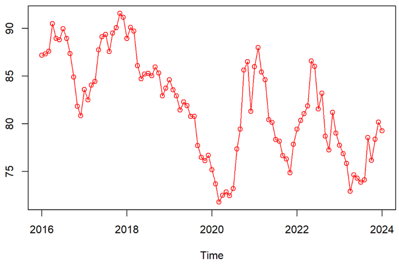
Figure 1: The trends of the US dollar index.

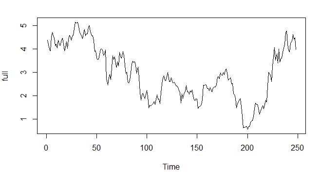
Figure 2: The trends of the US 10-year Treasury bonds.

As it is shown in the figure that the trend of the US dollar index is downward trend in general. It can be observed that the sequence of US 10-year Treasury bonds exhibits a pronounced linear increasing trend, it went down from 2004-2020 and rise up from 2020-2021.

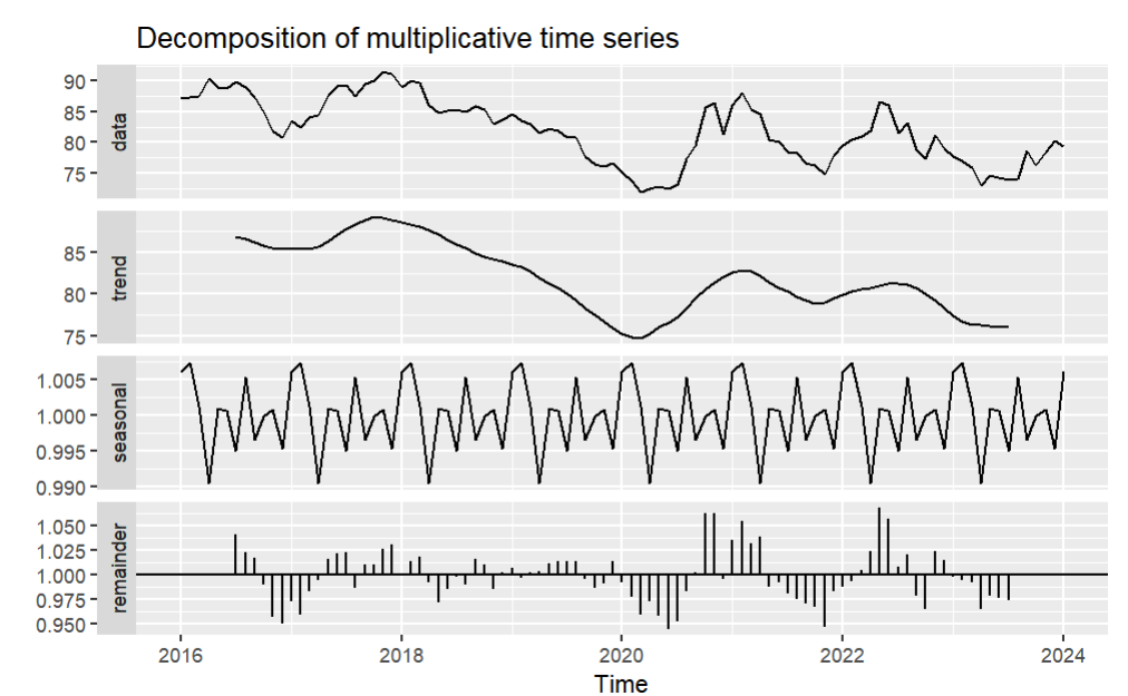
Figure 3: Decomposition of multiplicative time series.

The decomposition of multiplicative of time series can clearly show the trend, seasonal term, and remainder of the time series

And It can be observed from the trend of the original sequence that the current sequence is non-stationary. Therefore, this article performs differencing on the original sequence and performs ADF testing on the differenced original sequence. The differential sequence trend and ADF test results are shown in Figure 3-5 and Table 1.

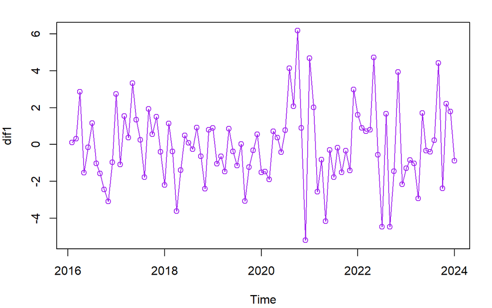
Figure 4: Differential sequence of US dollar index.

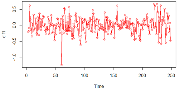
Figure 5: Differential sequence of US Treasury bonds.

Table 1: Augmented Dickey-Fuller Test.

The Table 1 show that the p value equals to 0.02409 and 0.01 which is smaller than 0.05, so the series is stationary.

After that it has to test the pure randomness, in order to ensure it is a non-white noise stationary sequence, this test is based on the value of p to judge whether it is pure randomness, and the alternative hypothesis is that the data is a non-white noise sequence. This means that, in contrast to the null hypothesis (H0) which might assume the data is white noise or has some other specific statistical property, the alternative hypothesis asserts that the data exhibits statistical characteristics that deviate from being white noise, indicating potential structure or patterns in the data.

Table 2 shows that the p value equals to 0.01383, which smaller than 0.05 which reject the null hypnosis’s and confirm that it is a non-white noise stationary sequence.

Table 2: Pure randomness test.

3. Empirical Result Analysis of ARIMA

3.1. Parameter Determination

Once the model orders are determined, the specific forecasting model can be identified. The practical implementation of this can be achieved through the auto.arima() function in R.

The ARIMA choose (0,1,0) since d is the differtiation order, if d=0, the series is not stationary. And usually when AIC, AICc and BIC are smaller the model is better. The results of parameter selection in this article are shown in Table 3.

Table 3: The results of auto ARIMA.

3.2. Model Significance Testing

The main purpose of model significance testing is to verify the validity of the model. A model is considered significantly effective mainly based on whether it extracts sufficient information. This can be achieved through the tsdiag() function in R.

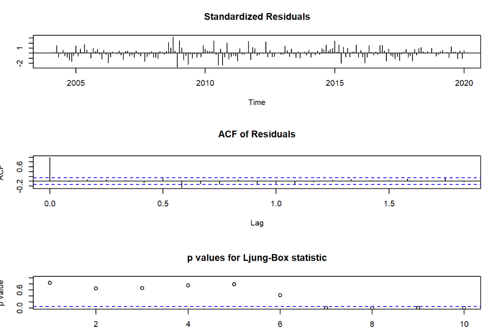
Figure 6: model Significance Testing of US dollar index.

According to the white noise test result graph in the figure 6, the P-values of the white noise test statistics after the 6th lags are significantly less than 0.05. Therefore, it can be concluded that the residual sequence of this fitted model does not belong to a white noise sequence, indicating that the fitted model is not significant. So, lets fitted the model with seasonal term for the US dollar index.

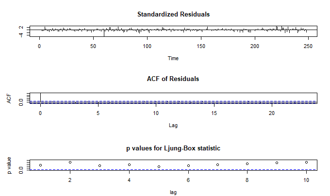
Figure 7: Model Significance Testing of US 10 years Treasury bonds.

And according to the white noise test result graph in the figure 7, the P-values of the white noise test statistics under various lags are significantly higher than 0.05. Therefore, it can be concluded that the residual sequence of this fitted model does belong to a white noise sequence, indicating that the fitted model is significant. which shows that the auto.ARIMA function is reliable for US 10 year Treasury bonds.

It can be seen that the ACF value is smaller than without seasonal term, it turns out to be a more precisely model for US dollar index to predict (see Table 4).

Table 4: The ARIMA model adding the seasonal term for US dollar index.

The red line in the figures 8-9 represents the observed values, the solid line represents the fitted values, the dark shaded area represents the prediction confidence interval with a confidence level of 80%, and the light shaded area represents the prediction confidence interval with a confidence level of 95%. It can be concluded that the trend of US dollar activeness in the future will be stable and around 80. And the US Treasury bonds trend will also be stable and around 4.

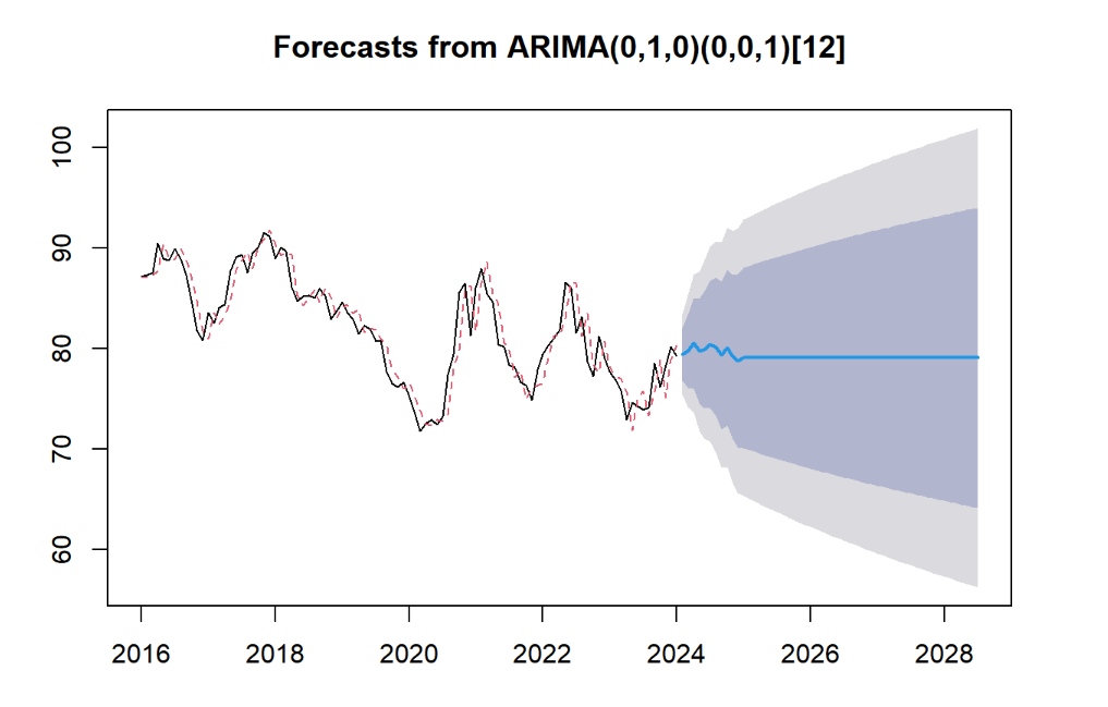
Figure 8: The prediction of US dollar index by ARIMA model.

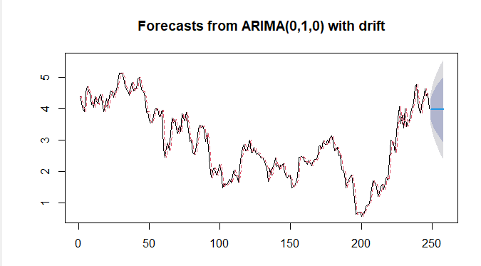
Figure 9: The prediction of US Treasury bonds by ARIMA model.

4. VAR Model

4.1. Determination of Lag Order

Using the VAR model to determine the lag order is crucial as it helps identify the appropriate number of past time periods to consider in the model, ensuring accurate forecasting and effective analysis of time series data [8-10].

Table 5: Select the lag order process.

From the above Table 5, the author can observe that in the AIC and SC tests, the SC test result is smaller. Generally, when the sample size is small, selecting lag orders of 1, 2, or 3 can yield better results. Hence the author chooses 1 for the lag value.

4.2. Stability Test

If the moduli of all the characteristic roots of the model are less than 1, or lie within the unit circle, then the model is stable. The table 6 shows 2 roots which both under 1, so the model is stable.

Table 6: The characteristic roots of the VAR model.

4.3. Impulse Response Analysis

In the VAR model, the Impulse Response Function (IRF) describes the reaction of other variables in subsequent periods when one variable in the system receives a unit impulse (i.e., an instantaneous shock). As the table 7 shows that when giving a shock to one of the variables and the other variable doesn’t show a strong reaction.

Table 7: Covariance matrix of residuals.

4.4. Residual Autocorrelation Analysis

The significance of autocorrelation test for residuals in VAR models lies in ensuring model adequacy. It verifies that residuals are independent over time, crucial for valid inference and prediction. Failure to do so indicates model misspecification or inadequate lag selection. As it shows in Table 8,the correlation of residuals between US Treasury bonds and US dollar index are pretty low. Hence, the model is effective.

Table 8: Correlation matrix of residuals.

4.5. Forecast by VAR Model of US Dollar Index

Finally, this article predicts the US dollar index based on the VAR model, and the results are shown in Figure 10.

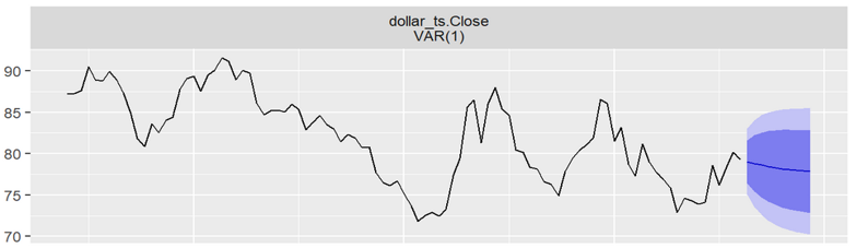
Figure 10: The trend of US dollar index base on VAR model.

5. Conclusions

The ARIMA model was used to predict the future trends of US dollar and US Treasury bonds separately, and the VAR model forecast the future trend based on their relationship. It was found that the correlation between the two was low. Taking this correlation into account, the future trends were predicted again, and the results were basically consistent with the previous ones, except for the US dollar index which VAR model predicts a slight downward trend in the future.

In the research process, the parameters of the ARIMA model were all set to ARIMA(0,1,0), but in actual situations, using other parameters might yield better prediction results. Additionally, the prediction method was relatively simple, which could lead to significant deviations from actual outcomes, and the VAR model had too few independent variables. Directions for future research improvements could include modifying the ARIMA model, such as incorporating seasonal factors, and comparing the results produced by different prediction models. When using the VAR model, more independent variables could be added to observe the impacts of different variables.

References

[1]. Huang Yuting & Xu Wei. (2023). Market Performance and Lessons from the Phase of the Federal Reserve's Pause in Rate Hikes. China Money Market (12), 49-51.
[2]. Wu Wu. (2021). Global Economic Outlook Improves, but the Foundation for Recovery is Relatively Fragile - Analysis of the World Economic Situation in the Second Quarter of 2021. Statistics Science and Practice (10), 4-7.
[3]. Anonymous. (2024). Recent Trends and Outlook of Financial Markets. Modern Finance Review (05), 38-40.
[4]. Ming Ming. (2023). Inversion of the US Treasury Bond Yield Curve and the US Economic Downturn. China Foreign Exchange (15), 64-68.
[5]. He Liping. (2024). Analysis of the Limited Impact of Federal Reserve Rate Hikes on the Current US Economy. International Finance (02), 29-37.
[6]. Luan Xi. (2022). Trends and Risks of US Treasury Bond Yields. China Foreign Exchange (22), 70-71.
[7]. Zhang Xiaobo & Fang Yuqi. (2023). Analysis of the Impact of US Treasury Bond Rates on the US Dollar Index. China Money Market (11), 36-39.
[8]. Liu Xiaoshu, Zheng Zhenlong. (2007). Verification of the predictive ability of commercial bank VAR model Contemporary Finance and Economics (8), 5.
[9]. Zheng Li, Duan Dongmei, Lu Fengbin, Xu Wei, Yang Cuihong, Wang Shouyang. (2013). Integrated prediction of pork consumption demand in China: empirical analysis based on ARIMA, VAR, and VEC models Systems Engineering Theory and Practice, 33 (4), 8.
[10]. Li Hana. (2022). VAR Model for Domestic Crop Price Prediction and Analysis, Chongqing University.
Cite this article
Yan,S. (2024). The Relationship Between US Dollar Index and US 10 Year Treasury Bond. Advances in Economics, Management and Political Sciences,124,64-72.
Data availability
The datasets used and/or analyzed during the current study will be available from the authors upon reasonable request.
Disclaimer/Publisher's Note
The statements, opinions and data contained in all publications are solely those of the individual author(s) and contributor(s) and not of EWA Publishing and/or the editor(s). EWA Publishing and/or the editor(s) disclaim responsibility for any injury to people or property resulting from any ideas, methods, instructions or products referred to in the content.
About volume
Volume title: Proceedings of the 8th International Conference on Economic Management and Green Development
© 2024 by the author(s). Licensee EWA Publishing, Oxford, UK. This article is an open access article distributed under the terms and
conditions of the Creative Commons Attribution (CC BY) license. Authors who
publish this series agree to the following terms:
1. Authors retain copyright and grant the series right of first publication with the work simultaneously licensed under a Creative Commons
Attribution License that allows others to share the work with an acknowledgment of the work's authorship and initial publication in this
series.
2. Authors are able to enter into separate, additional contractual arrangements for the non-exclusive distribution of the series's published
version of the work (e.g., post it to an institutional repository or publish it in a book), with an acknowledgment of its initial
publication in this series.
3. Authors are permitted and encouraged to post their work online (e.g., in institutional repositories or on their website) prior to and
during the submission process, as it can lead to productive exchanges, as well as earlier and greater citation of published work (See
Open access policy for details).