1. Introduction

There are numerous characteristics associated with time series data, which is why it is essential to decompose a time series into different components that represent the various underlying pattern categories. The major components of time series patterns include trends, seasonal variations, and cycles. Therefore, the time series decomposition is necessary for understanding time series better and making more accurate forecasting. Today’s high sampling rates provide interfaces for high-frequency data (like daily, hourly, and minute-by-minute data), resulting in various seasonal time series that include numerous patterns in many real-world data sets [1]. To better understand the structure of time series data, it is essential to eliminate the seasonal data because the time series data has always been complicated by seasonal patterns. In this study, the author will explore a detailed overview of four popular decomposition methods: Classical, X11, SEATS, and STL, and discuss their application, strengths, and limitations. The R package “seasonal” is used to conduct these decompositions on National Oceanic and Atmospheric Administration (NOAA) Climate Data.

Time series decomposition is a statistical technique of breaking time series information down into its individual components. Three primary elements discussed are the trend cycle, seasonal variations, and the remaining components that address other aspects of the given data over a given period. The separation of this type of regular seasonal pattern allows for a correct specification of the structure of the time series [2]. To understand the nature of these sequences, all such patterns are removed and even as preparation for future work, any condition is forecasted and removed from the data. Any figures obtained after processing the raw data by subtracting all seasonal fluctuations are called “seasonally adjusted.” This technique is very important in the identification of patterns in data, making predictions, and identification of outliers.

The majority of people use two primary models, which are referred to as the additive model and the multiplicative model [3]. In an additive model, a time series can be expressed as a sum of its components: trend, seasonal, and noise (residual).

\( \text{ Y(t) = Seasonal(t) + Trend(t) + Residual(t) } \) (1)

Where Y(t) is the time series data at time t. Seasonal(t) is the seasonal component, Trend(t) is the trend-cycle component, and Residual(t) is the remainder component at time t. This model is most suitable especially when the size of a seasonal variation is invariant with the size of the time series. When the volume of the seasonality corresponds to that of the time series, the multiplicative model is effective [4]. The multiplicative model of time series assumes that various components interact proportionally, and time series can be represented as the product of its components:

\( \text{ (t) = Seasonal(t) × Trend(t) × Residual(t) } \) (2)

2. Methodology

In this research, the methodology includes an analysis of four decomposition techniques. These include the Classical method, X11, SEATS, and STL Decomposition. This paper employed the NOAA’s average global land-ocean surface temperature (NOAATMP) time series, which is a monthly project that covers January 1980 to July 2024. NOAATMP dataset contains a collection of temperatures distributed across space globally every month since 1880 (NOAA National Centers for Environmental Information). The land-based data is therefore derived from weather stations that record near surface or air temperature while in the ocean, this type of information is from ships or drifting buoys that record sea surface temperature (SST).

The data has been prepared and analyzed with the help of R programming. R is a language which is used as a tool for data analysis. R is open source and has a huge collection of packages with several functions for the analysis of data [5]. For this research, the following R packages were used: “forecast”, “ggplot2”, and “seasonal.” The “forecast” package provides functionality for forecasting time series data. The “ggplot2” package offers functions for the visualization of the data, and the “seasonal” package offers key functions for the decomposition of the time series data, which are mandatory for the proposed model. If the “seasonal” package was not installed earlier in R, then it can be installed with the help of the command install.packages(“seasonal”).

The data is available in the database NOAATMP when downloaded into a CSV file consisting of Dates and Anomalies in the temperature for the 1901–2000 average. The default time series plot is plotted with the help of ggplot() function of the package “ggplot2” to explain deviations in temperature from 1980 to 2024. The output of the ggplot() is shown in Figure 1.

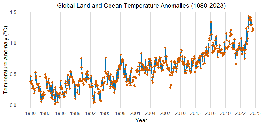
Figure 1: Global Land and Ocean Temperature Anomalies time series (1980-2024).

2.1. Classical Decomposition

The classical decomposition technique is one of the earliest approaches that have been utilized in the analysis of time series data. The method assumes that a time series can be expressed as a sum of its components: trend, seasonal, and residual [6]. It also presumes that seasonality remains unchanging, while this presents a challenge for climate records because seasonal patterns can change with time [7]. There are two ways to do classical decomposition with an additive or multiplicative decomposition model.

This paper utilizes the autoplot() function in R, provided by the “ggplot2” package, to plot the result of both additive and multiplicative classical decompositions. This function provides separate plots for the trend, seasonal, and remainder (residual) components, making it easier to interpret these aspects of the time series. Figures 2-3 show the decomposition results for the additive and multiplicative decomposition.

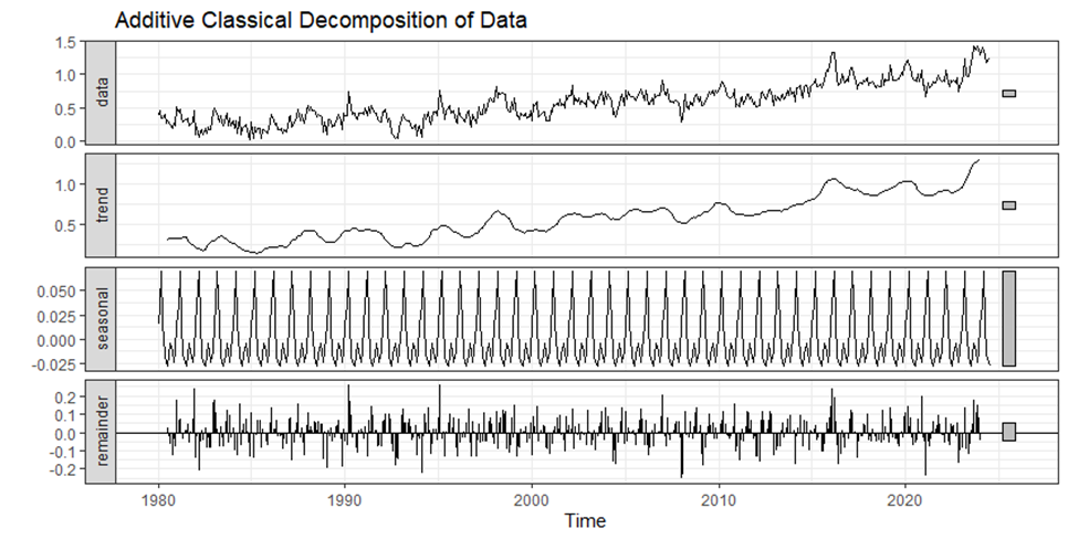
Figure 2: Additive Classical Decomposition of NOAATMP time series data.

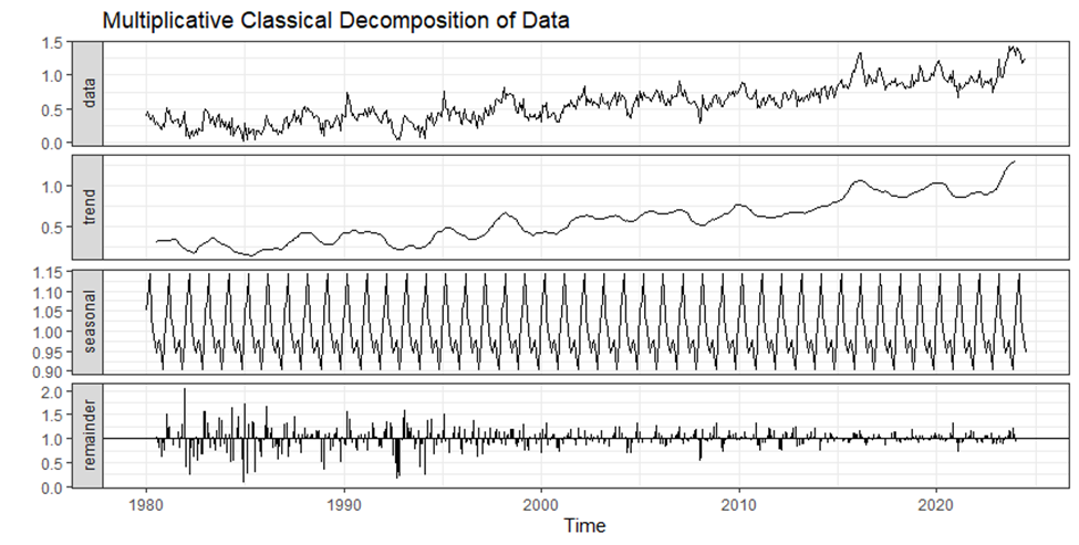
Figure 3: Multiplicative Classical Decomposition of NOAATMP time series data.

2.1.1. Analysis

In classical decomposition, both methods for addition and multiplication are used to decompose NOAA global land-ocean surface temperature (NOAATMP) time series into trend, seasonal, and remainder components. The trends that are derived from both decompositions express an increase in global temperature starting from 1980 to 2024 showing the effects of climate change. Two trends, which are identical in showing the increase consistent with global warming, are displayed for each method with their significant difference in seasonal and remainder fluctuations. The signs of additive decomposition suggest that the remainder is rising, which implies the growth of the absolute variability of temperature anomalies over time. On the other hand, if the remainder of the multiplicative decomposition is smoother, then the relative variability is expected to be less variable while the absolute variations are getting near the warming signal magnitude.

When comparing and contrasting the two decompositions, elements of variability in long-term climate evolution can be brought into focus. The additive model is less able to interpret and accommodate changing seasonal effects, and for this reason, short-term fluctuations and anomalies are more pronounced. Whereas the multiplicative model eliminates such variance by incorporating interaction terms of the seasonal and the trend. Climate information is a function of several factors that are complicated and interconnected, hence this relationship is important.

2.1.2. Application

In economics as well as environmental science, classical decomposition is frequently employed for recognizing seasonal patterns in data. It is appropriate for exploratory data analysis in production characterized by constant seasonal cycles. For instance, temperature variations measured monthly may be analyzed by researchers using this technique to reveal cyclical shifts and seasons. Classical decomposition is often used for educational purposes because of its simplicity.

2.1.3. Strengths

Classical decomposition is known for its simplicity. Because of its simple structure, it is great for beginners to perform time series analysis. It provides modeling flexibility for users by allowing both additive and multiplicative decomposition choices for easier understandability. Interpretability of decomposed time series into trend, seasonal, and remainder components makes it easier to observe and understand clear patterns in the data.

2.1.4. Limitations

Classical decomposition methods assume fixed patterns in the seasonal component that repeat from year to year. For longer series and time series with changing patterns, it can produce misleading conclusions [6]. It assumes constant seasonal effects and has less effectiveness in the case of complex or evolving seasonal and trend components such as climate data because of evolving seasonality and complex climate cycles. As shown in Figures 2-3, trend estimates for the first and last observations are not available. Classical decomposition is sensitive to outliers, and it might distort the results. This may lead to inaccurate conclusions for extended periods of a complex, changing climate. Therefore, newer methods have been designed to overcome these limitations.

2.2. X11 Decomposition

X11 decomposition is based on the classical decomposition method, and it was first introduced by the US Census Bureau and further developed by Statistics Canada. It offers some extra features and eliminates the limitations of the classical decomposition method. For the X11 decomposition, the author has used the “seasonal” package in R. The function seas() perform seasonal decomposition using the X11 method. Seasonal adjustments to time series data are commonly plotted using this technique. Figure 4 shows original data, seasonal components, trends, and irregular components after a decomposition using the X11 decomposition method.

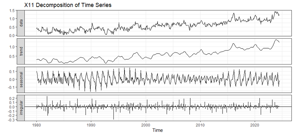
Figure 4: X11 Decomposition of NOAATMP time series.

2.2.1. Analysis

A combined plot shows a more detailed plot that overlays multiple components of the time series. The trend-cycle component is overlaid by using the forecast:autolayer() function on the trend component. The x11 decomposition is smarter in handling seasonal patterns. This method is more helpful in analyzing climate data because seasons are not as predictable as they used to be. There is a visible pattern of a steady upward rise in temperature due to global warming. Global warming is not just a theory but a reality which can be seen on the trend line. There are also little ups and downs in the temperature anomalies, probably because of things like El Niño or big volcano eruptions. Volcanoes including Mt. Krakatoa in Indonesia, Mt. Pinatubo in the Philippines, and El Chichón in Mexico caused the blocking of sunlight with its dust and sulfate aerosols [8]. Temperature fluctuations throughout the year were captured by seasonal components. X11 decomposition uses moving averages to smooth out these seasonal patterns.

The remainder component in X11 decomposition shows irregular variations or noise in the data after removing the trend and seasonal components. This method has isolated the short-term anomalies and extreme events in climate data more clearly. From this, the impact of overall temperature trends could be better understood. Unusual patterns and spikes indicate significant climate events like El Niño or volcano eruptions affecting the Earth’s climate.

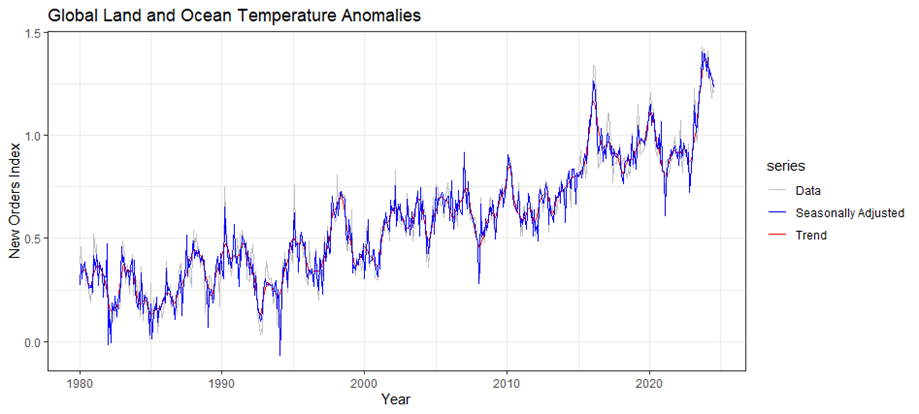
Figure 5: Time series for NOAATMP: original data (gray), trend-cycle component (red), and seasonally adjusted data (blue).

The seasonal sub-series plot is used to visualize the seasonal component extracted from the X11 decomposition [9]. The function ggsubseriesplot() illustrates how seasonal effects vary across different years and periods. As for the X11 decomposition, the plot of the seasonal sub-series is given in Figure 6. This shows a detailed view of recurring patterns in the climate data within each year. This visualization can help reveal any shifts or changes in the seasonal pattern, such as whether some months are becoming warmer or cooler over time. For instance, if the plot indicates that summer months have been consistently getting hotter in recent years, it may indicate changing seasonal temperature patterns due to global warming.

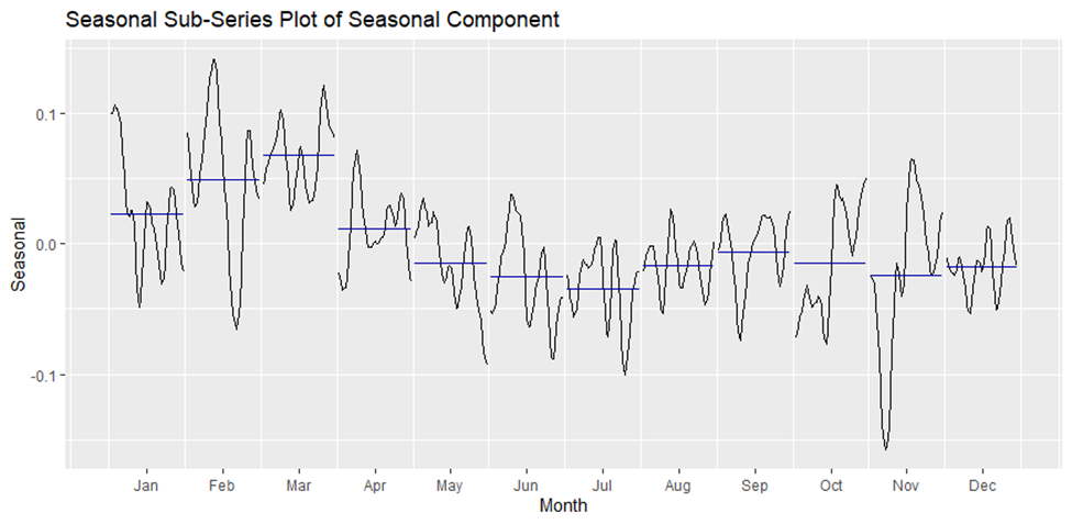
Figure 6: Seasonal sub-series component from the X11 decomposition.

2.2.2. Application

The X11 decomposition method is widely used for analyzing economic and financial context data. It is an effective time series analysis tool, but it should be used carefully and with other analytical tools for more complicated or changing time series [6]. It is most useful in dealing with the problem of the seasonality of data, to allow some people to make comparisons of one period with another free from the influence of the seasons.

2.2.3. Strengths

One of the key strengths of the X11 decomposition is its flexibility. It is most appropriate for all types of seasonality, these being the additive and multiplicative types. This makes it suitable for a wide range of datasets like climate data, which has complex seasonality patterns. It can perform automatic data processing and therefore minimizes human input while being easy to control for time series use. It provides reliable results with user-friendly interaction. This method is known for its robustness, as it can detect outliers in data. The changes in level and detection of the outliers make X11 sufficiently powerful for use in real datasets containing anomalies.

2.2.4. Limitations

This decomposition technique has several sub-processes and phases, which make it extra complex and less easy to understand. Sometimes it might have biases at the early or closing periods of the series, which makes it cumbersome in terms of predicting characteristics. Another limitation of X11 decomposition is the amount of data requirements. There must be much information to get probable outcomes. The time series decomposition may depend on the points at which it starts and finishes. The interpretation of cyclical components can be subjective and specific to the application.

2.3. SEATS Decomposition

Statistical SEATS (Signal Extraction in ARIMA Time Series) decomposition is a method of analyzing the time series data to identify seasonal components. SEATS decomposition was developed at the Bank of Spain [6]. This is widely used among government agencies and researchers who use it to analyze and adjust for seasonal effects, thereby identifying clear trends and cycles hidden in the data. This technique is particularly relevant when working with quarterly or monthly time series, thus making it an essential instrument for economists and analysts aiming at recognizing changes in economic activities over time [10]. For SEATS decomposition, the seas() function from the “seasonal” package is used with the time series data “climateDataSeries” as an argument. Another function autoplot() is used for plotting the extracted components after the SEATS decomposition. The Figure 7 shows the different components after SEATS decomposition.

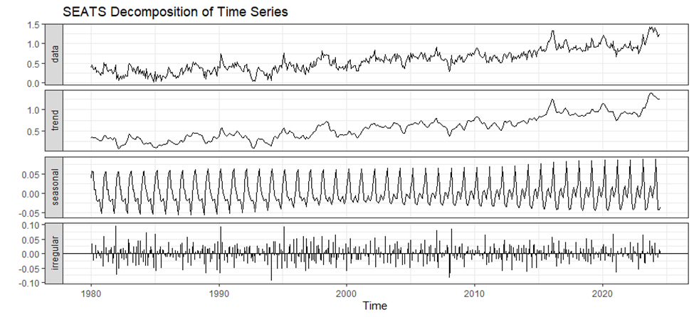
Figure 7: SEATS decomposition of NOAATMP time series.

2.3.1. Analysis

SEATS decomposition takes advantage of AutoRegressive Integrated Moving Average (ARIMA) models to decompose complex climate change time series data into trend, seasonal, and irregular components. It helps to analyze both long-term trends and seasonal patterns. Using ARIMA techniques, SEATS can identify subtle shifts in global temperatures over time, which can be seen in the above trend component.

Utilizing ARIMA models, the periodic structure of climate statistics was separated into seasonal fragments that express shifting seasonal characteristics more efficiently than typical approaches. The amplitude or timing alterations cause the seasonal component’s regular temperature fluctuations. After excluding trend and seasonal components, the irregular changes are shown by the residual element. By making it easier to identify unusual temperature events or short-term deviations from the expected patterns, it provides a more accurate and smoother remainder series.

2.3.2. Application

Analysis and forecasting of economic data are widely undertaken using SEATS decomposition technique. The cyclical movement in economic variables such as GDP, inflation rate, and employment levels are explained by changes in these variables’ values. Thus, this is the most appropriate method for transforming time series data to remove seasonal variations that facilitate comparisons across different time periods. The principal application of SEATS is in the transformation of a time series to eliminate personalities. Moreover, by decomposing the system into its seasonal components and modulating them separately, SEATS can also be employed for forecasting future values of time series data. Governments and organizations use SEATS to assess the impact of economic policies by evaluating seasonally adjusted data. Removing the seasonality effects can assist in estimating the real impacts of policies, thus allowing informed decision-making facilities by more accurate understanding of economic patterns.

2.3.3. Strengths

One of the key strengths of the SEATS decomposition is its robustness. SEATS is not sensitive to different forms of irregularities in the data, and hence suitable for utilization in real datasets that might contain anomalous points. Unlike the naive method, the trading day’s variations and other known factors are considered and applied to seasonality decomposition. Integration with ARIMA Models: SEATS is, in fact, well aligned to ARIMA models and can accurately model time series data in seasonally adjusted or non-seasonal methods. It is a widely accepted decomposition technique for time series forecasting, and it is now a standard method recognized and applied by many government agencies and is commonly employed as a technique for economic analysis.

2.3.4. Limitations

One of the main drawbacks of the SEATS decomposition is the requirement of data for better prediction. It is best suited for quarterly and monthly data but can be used to some extent for other types of data which are weekly, daily, and even multi day. It may also take some time to apply and comprehend, especially if one is not conversant with the procedures of using ARIMA models and the procedures of seasonal decomposition. Another limitation is SEATS takes the approach that the seasonal pattern does not change much over the years, which again may produce inaccurate estimates. Lastly, SEATS can suffer from end-point bias. This will affect the accuracy of the model’s prediction at the beginning or end of the time series, which compromises the validity of any forecast that is derived from the model.

2.4. STL Decomposition

The Seasonal and Trend decomposition using Loess (STL) decomposition is performed by using stl() function in R. This technique is powerful and adaptable, permitting the segmentation of seasonal, trend, and irregular components of time series data [6]. The periodicity of the seasonal component can be achieved by using the s.window = “periodic” parameter, whereas robust = TRUE option provides less sensitivity towards outliers, thus increasing the dependability of outputs. The Figure 8 shows the STL decomposition of NOAATMP time series into its trend, seasonal, and irregular (random) components.

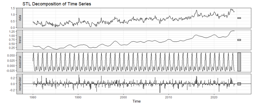
Figure 8: STL decomposition of NOAATMP time series into its trend, seasonal, and irregular (random) components.

2.4.1. Analysis

STL decomposition is a versatile and strong methodology for datasets with non-linear tendencies and dynamic seasonal trends. It can perform LOESS smoothing to get seasonality, trend, and remainder components of time series data. Here, the trend component represents globally smooth and non-linear alterations in land-ocean surface temperatures. This part of the temperature series shows its long-term way, indicating an overall increase. Because of its flexible nature in smoothing, STL can also capture complex variations over time, which makes it ideal for representing minor changes in climatic patterns.

The seasonal component in STL is estimated using a flexible LOESS method that is capable of accommodating changing amplitudes and timings of seasonal effects. In the case of NOAATMP time series, the seasonal component can depict, with good accuracy, how temperature fluctuations differ from month to month during a year. Analyzing climate data where there might be transformations in seasonal effects consequent upon global warming or any other circumstance highly benefits from STL’s capacity to adapt to changes in periodic patterns over time. In the STL decomposition, the remainder component (or residuals) captures the irregular fluctuations left after the trend and seasonal effects have been removed [11]. Consequently, the application of LOESS smoothing in the STL results in more stable and cleaner remainder series that are good at elucidating anomalies and outliers. That way, it helps to understand short-term deviations or unusual temperature observations by contextualizing them with long-term trends and seasonal behaviors.

2.4.2. Application

With STL, time series data is broken down into a trend component, a seasonal component, and a residual component respectively. It is widely used in various sectors like economics, weather forecasting, and business analytics [12]. It is suitable where information varies seasonally or experiences temporal fluctuations in seasonality levels.

2.4.3. Strengths

The main strength of STL decomposition is its flexibility in handling different time series patterns. It can contextualize both additive and multiplicative seasonality, as well as nonlinear trends [2]. The method is robust, it can work with outliers and missing data, which is a great advantage for real-world applications. It can handle variations in time series automatically. As a result of eliminating trading-day effects and other known predictors for holidays to return to a precise breakdown. To manipulate ‘trend-cycle smoothness’ there are parameters provided to users, which also allow handling of the seasonal components, according to the properties of certain data. This allows users to extend the decomposition to their needs. It also provides computational efficiency. In large data sets as well as in real-time applications, this can perform well without requiring a lot of computational power.

2.4.4. Limitations

There are some limitations worth mentioning for the STL decomposition method. Unlike some techniques (such as X11), STL does not make variations regarding trading days or calendars, but data requires further pre-processing. The use of LOESS smoothing in STL can also be computationally complex, especially when working with large datasets, which may make the process time-consuming. STL is also sensitive to parameters. Adjusted outputs may vary based on several factors, including parameter values (e.g., smoothing factor) that would require fine-tuning until the best outcome is reached. Finally, although the main purpose of STL is to perform additive decomposition, although it can also be modified to multiplicative decomposition, it may not be applicable to every type of time series information.

3. Conclusion

In conclusion, the empirical investigation of Classical, X11, SEATS, and STL decomposition methods was performed using the NOAA National Climatic Data Center’s global land-ocean surface temperature time series from January 1980 to August 2024. This dataset comprises information on the monthly temperature record, over land, through weather stations, and over sea, through ships and drifting buoys. The research adopted the R programming language with the aid of packages inclusive of “forecast” for time series analysis, “ggplot2” for graphical analysis, and “seasonal” for performing the decompositions.

Classical decomposition worked well for simple and less complex analyses but could not be applied to more complicated data. On the contrary, X11 had its limitations in terms of complexity and sensitivity to data conditions, although it was applicable to a variety of seasonal patterns. Furthermore, SEATS decomposition performed well with irregular components and complex patterns but was too demanding when it came to stationary assumptions. Despite requiring precise parameter tuning as well as additional preparation, it turned out that STL decomposition was the most flexible one since it addressed non-linear trends or changing seasonal effects more effectively. Therefore, this study has established that the choice of an appropriate method of comparative decomposition is largely dependent upon specific data characteristics and research objectives, given the significant effect this choice can have on analysis accuracy and forecast reliability.

References

[1]. Bandara, Kasun, et al. (2021). MSTL: A Seasonal-Trend Decomposition Algorithm for Time Series With Multiple Seasonal Patterns. Cornell University.
[2]. Dudek, Grzegorz. (2023). STD: A Seasonal-Trend-Dispersion Decomposition of Time Series. IEEE Transactions on Knowledge and Data Engineering, 35 (10), 10339-10350.
[3]. Duncan, Richard P., and Ben J. Kefford. (2021). Interactions in Statistical Models: Three Things to Know. Methods in Ecology and Evolution, 12(12), 2287-2297.
[4]. Proietti, Tommaso, and Diego J. Pedregal. (2022). Seasonality in High Frequency Time Series. Econometrics and Statistics, 27, 62-82.
[5]. Kabacoff, Robert. (2022). R in action: data analysis and graphics with R and Tidyverse. Simon and Schuster.
[6]. Hyndman, Rob J., and George Athanasopoulos. (2018). Forecasting: Principles and Practice. 2nd ed., OTexts.
[7]. Liu, Xiao, and Qianqian Zhang. (2024). Combining Seasonal and Trend Decomposition Using LOESS With a Gated Recurrent Unit for Climate Time Series Forecasting. IEEE Access, 1.
[8]. Predybaylo, Evgeniya, et al. (2017). Impacts of a Pinatubo‐size volcanic eruption on ENSO. Journal of Geophysical Research Atmospheres, 122(2),925-947.
[9]. Tebong, Njogho Kenneth, et al. (2023). Application of Deep Learning Algorithms to Confluent Flow-rate Forecast With Multivariate Decomposed Variables. Journal of Hydrology Regional Studies, 46, 101357.
[10]. Liu, Xinyang, et al. (2023). Impact of Decomposition on Time Series Bagging Forecasting Performance. Tourism Management, 97, 104725.
[11]. NOAA National Centers for Environmental Information. Climate at a Glance: Global Time Series. August 2024. Retrieved from https://www.ncei.noaa.gov/access/monitoring/climate-at-a-glance/global/time-series.
[12]. Ollech, Daniel. (2021). Seasonal Adjustment of Daily Time Series. Journal of Time Series Econometrics.
Cite this article
Huang,R. (2024). Differential Analysis Based on Different Decomposition Methods of Time Series. Advances in Economics, Management and Political Sciences,124,121-132.
Data availability
The datasets used and/or analyzed during the current study will be available from the authors upon reasonable request.
Disclaimer/Publisher's Note
The statements, opinions and data contained in all publications are solely those of the individual author(s) and contributor(s) and not of EWA Publishing and/or the editor(s). EWA Publishing and/or the editor(s) disclaim responsibility for any injury to people or property resulting from any ideas, methods, instructions or products referred to in the content.
About volume
Volume title: Proceedings of the 8th International Conference on Economic Management and Green Development
© 2024 by the author(s). Licensee EWA Publishing, Oxford, UK. This article is an open access article distributed under the terms and
conditions of the Creative Commons Attribution (CC BY) license. Authors who
publish this series agree to the following terms:
1. Authors retain copyright and grant the series right of first publication with the work simultaneously licensed under a Creative Commons
Attribution License that allows others to share the work with an acknowledgment of the work's authorship and initial publication in this
series.
2. Authors are able to enter into separate, additional contractual arrangements for the non-exclusive distribution of the series's published
version of the work (e.g., post it to an institutional repository or publish it in a book), with an acknowledgment of its initial
publication in this series.
3. Authors are permitted and encouraged to post their work online (e.g., in institutional repositories or on their website) prior to and
during the submission process, as it can lead to productive exchanges, as well as earlier and greater citation of published work (See
Open access policy for details).