1. Introduction

For most industries nowadays, from manufacturing to commerce, Inventory is always an inevitable topic to discuss. It not only benefits the company itself but also has a great impact on sales and customers. Inventory plays a very important role in supply chains because of several functions it can perform. When some industries are producing some products with economic batch requirements to minimize the cost, usually there will be a difference between the economic batch quantity and customer-ordered quantity. Inventory could be used to fill in the inconsistency. In addition, the manufacturing speed is inconsistent with the customer’s needs at times due to factors such as seasonal changes. Therefore, the inventory is used to balance it. Additionally, inventory also serves to mitigate the risk of unforeseen circumstances such as fluctuations in customer demand and supply replenishment [1].

Due to the irreplaceable functions that inventory serves, effective inventory management becomes crucial in saving both space and cost. Some products may have a limited shelf life, which is also a factor to consider. I decided to delve deeper into this topic to better manage and understand the inventory. Since most of the research is either business analysis or machine learning model prediction, there are few researchers who utilize both methods simultaneously. So I decided to use both methods simultaneously to compare the results from different angles and perspectives, and then to see what results data scientists and business analysts get in common, as well as the advantages and disadvantages of both methods. In this paper, a dataset of a grocery store’s inventory will be used. Then ABC analysis and linear regression model are selected to analyze the data. Both methods are common and widely used in their respective fields [2][3]. ABC analysis is for business analysis and linear model is for machine learning or data science. Since the data isn’t too complicated for this dataset, these two methods are appropriate here. The analysis is trying to find out if the inventory is good or experiencing some issues such as increasing cost, excess inventory, stockouts, etc. And then give some pieces of advice for the grocery store about managing the inventory. This research can serve as an example of inventory analysis, providing a logical framework for others to apply in their own examination of different inventory data. By doing so, more companies can identify potential inventory problems at an earlier stage.

2. Methodology

2.1. Histogram

The histogram shows the overall distribution of all the columns in the dataset [4]. It is used to get some general ideas about the dataset. From Figure 1, the store figure and saleDate figure are continous data. Meanwhile, other figures don’t and they look more like classification information. So the research will focus on those two trends next.

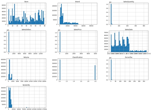
Figure 1: Histogram of the dataset

2.2. Correlation Matrix Heatmap

The purpose of the correlation matrix is similar to the histogram, to give us an overview of the dataset so we can have some ideas to build the linear regression model next. What’s different is that the correlation matrix shows the relationship between each two columns of data [5]. If the value approaches 0, it indicates a weaker relationship between the two data sets. A value of 0 signifies no relationship at all between the two values. As the value gets closer to 1, it suggests a stronger positive correlation between the two data sets. Conversely, if the value is closer to -1, it indicates a stronger negative correlation between the two data sets.

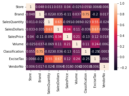
Figure 2: correlation matrix of the dataset

From Figure 2 shown above, it’s not hard to notice that sale quantity, sale dollar, and excise tax have the most positive relation. Brands and classification are also one of the most positively related pairs, but since they are not continuous data, are not considered in the linear regression model. Although excise tax has different values, the ratio is fixed most of the time. Since sale dollar = sale quantity * sale price, the linear regression next is still going to focus on the sale quantity and sale price.

2.3. Linear Regression

After the overview, the first method used in the paper is linear regression, which is commonly used in predicting the trend. In general, a linear regression model can be interpreted as finding a line that fits all the data distribution best. To achieve this, a gradient descent algorithm is used to minimize the square error cost function [6]. If the data is complicated, linear regression can also have multiple dimensions to fit the data. In this paper, the linear regression model is utilized to analyze two trends: sales quantity and sales price.

For sale quantity, the data need to be cleaned by grouping by date and sum up the quantity for the specific date. By fitting the linear regression model, we are able to get Figure 3.

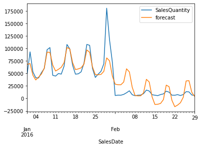
Figure 3: linear regression model for sale quantity

By testing this result, the R^2 score is 70.57%. In this case, the accuracy is high enough. Firstly, based on the data, it is evident that there is a significant increase in the quantity sold at the end of January compared to other times. It could potentially lead to overfitting if abnormal data is excessively accommodated. Therefore, disregarding that particular set of data may be a prudent choice in this scenario. [7]. In addition, the January data differs significantly from the February data, which introduces more volatility and variability into the dataset. This complicates the task of making accurate predictions. Therefore, it is reasonable to prioritize stability for future predictions over absolute accuracy in this case. Another reason is that despite the abundance of data in the dataset, there are only 60 observations after grouping and summing due to the dataset covering a time period of only two months. With such a limited number of observations, it is difficult to obtain a highly precise and accurate model..

After the linear model is scaled, the next step is applying the model to predict the next few months. Figure 4 shows the figure for the prediction.

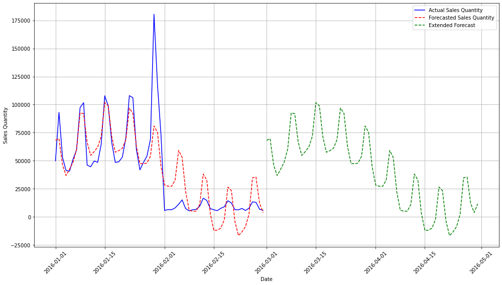
Figure 4: extended prediction for sale quantity

So even though the accuracy is not very high, the trend predicted is still very good for such a noisy dataset. With more data collected gradually, the result will definitely be better.

The sale price is similar to the sale quantity. The only difference with the above analysis is changing the sale quantity to the sale price and finding out the mean of price instead of summing up. The figure of the linear regression model for the sale price is shown below in Figure 5.

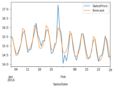
Figure 5: linear regression model for sale price

The trend for this figure is much more stable than the previous one. This one also has a higher accuracy of 80% for the R^2 score. The sale price for January is similar to the sale price for February. Except for the anomaly at the end of January, the rest are fitted very accurately. So the next step would be extending the forecast to predict the sale price for the next few months. Figure 6 next shows the prediction. As expected, since the data and the model have less turbulence, the predicted result showed a more stable and smooth trend.

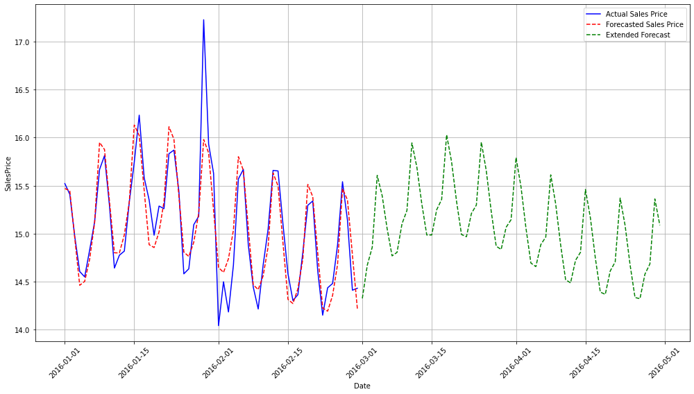
Figure 6: extended prediction for sale price

2.4. ABC Analysis

ABC analysis is primarily utilized to assess efficiency and allocation, and it is widely employed in daily sales and management issues. By conducting ABC analysis, a business can optimize its resource utilization [8]. The main idea of ABC analysis is to divide the cumulative frequency of the curve into three levels, the corresponding factors are divided into three categories.The first category, factor A, is defined as the most influential factor, occurring with a frequency of 90% to 100% of the time. The second category, factor B, is defined as the second most influential factor, occurring with a frequency of 70% to 90% of the time. The third category is factor C, which is defined as a generally influential factor and occurs with a frequency below 70%[9]. The purpose of applying ABC analysis in this paper is to help determine which segments or factors should gain more attention, thus improving sales efficiency and optimizing sales or inventory structure. For this dataset, it is expected some new management strategy that can be obtained from the analysis if the management is found to be inadequate.

In this case, some common statistical features will be analyzed and then the brand will be used to calculate the frequency they showed in the dataset and split them into three groups A, B, and C. The first quartile is obtained as 238 and the mean is 1015. So factor C is set to below 200, factor B is set to 200-1000, and factor A is set to 1000 above. So the frequency is roughly equal to 90%-100%, 70%-90%, and 0-70% accordingly. Figure 7 below shows the result. The quantity sold above average is only 572 brands, and the rest around 7000 brands are below average. Group A only takes 7.50% of all brands. The majority of brands are in Group C, which is 72.24%.

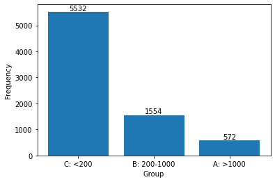
Figure 7: ABC analysis based on brand frequency

Figure 8 shows the result for the total sales of these three groups. Even though only 572 brands are in Group A, the amount of the sales is the majority of all the sale money earned, it’s 6.3 times larger than Group C. So the company should shift the focus to Group A and reduce some stock from Group C. Many brands only sold one quantity. Since they cannot be sold, stock for them might be a problem.

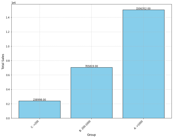
Figure 8: Total sales for each group

After verifying the stock-keeping unit (SKUs), it’s more clear to see that there’s a problem with inventory. While Group A brands earned around 60% percent of all profits, the SKUs for it are only 6%. Group C brands earned only 1% of all profits but it has 55% SKUs. the detailed results are in Figure 9.

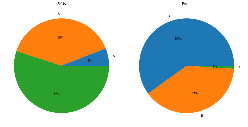
Figure 9: ABC analysis with SKUs

3. Discussion

The paper mainly focuses on two methods which are linear regression and ABC analysis. Both methods have different emphases. Linear regression is focused on utilizing historical data to predict future trends by identifying patterns in the data. ABC analysis focuses on the weight of each category or brand, and is utilized to determine the optimal stocking levels for different products. For this dataset, both methods provide insights into the situation of the inventory. In linear regression, it can be seen that the trend is decreasing for both sale quantity and sale profit. This mirrors the issue highlighted in the ABC analysis, where it was found that a majority of brands were not selling well yet still occupying inventory space. This could potentially be a contributing factor to the declining sales. However, in this case, the ABC analysis provides more comprehensive information compared to linear regression. The regression model only utilized two months of data and may not account for potential turbulence or unforeseen circumstances, such as holidays or seasonal changes. Two months of data may not be sufficient to accurately predict these changes. However, this does not necessarily indicate that ABC analysis is a superior method, as different cases and datasets could yield varying results. And with the recording of more data from this company, the performance of linear regression would significantly improve. At last, it can be concluded from two methods that the company should reduce the stock for items with a sales frequency of less than 200 times over a two-month period, especially if the sales frequency is only 1. Then the company should shift the attention to those brands sold very well in group A.

4. Conclusion

This paper investigated linear regression and ABC analysis and then applied these two methods to analyze the inventory of a company. Both approaches were effective in identifying the company's issues, with ABC analysis providing more detailed insights in this particular case. It showed that most products in inventory didn’t sell well and occupied the space meanwhile. It also recommended that the company should prioritize understanding which products are essential and which are not. The ABC analysis gives one of the reasons that the linear regression shows the company’s sales are declining. The linear regression here is also a good tool to verify that the company is on the right track and direction. Unfortunately, due to insufficient data, the dataset exhibits a high degree of turbulence, resulting in limited accuracy. However, we are still able to discern the overall trends provided by the linear regression model. With more and more data added, the linear regression could show more useful information. In this case, both methods play their parts well. For future research, the company should consider gathering additional data and continuing to monitor both the ABC analysis and linear regression.

The research proposed that the linear regression and ABC analysis are both able to spot the problem of an inventory. The advantage of linear regression is to keep tracking of the data as the data are updated and make sure the actions the company takes can positively affect future trends. On the other hand, ABC analysis is unable to keep tracking the data as the data keeps updating, but it emphasizes which brands should the company focus on and which brands are redundant. This information cannot be told from linear regression. However, the two methods might not be comprehensive enough. It is just able to spot the problem and provide a general solution. But for some specific actions that need to be taken to solve the problem, require more research and analysis methods such as economic order quantity analysis, reorder point, and lead time analysis to achieve it [10]. Then we can also use the data that is assumed after these actions are taken to predict the future trends to see if the actions are effective. With more angles and perspectives the analysis of the inventory could be more persuasive and comprehensive.

References

[1]. Brewer, A. M., Button, K. J., & Hensher, D. A. (2001). Handbook of Logistics and Supply-Chain Management. Elsevier.
[2]. Shakeel, R., & Siddiqui, D. A. (2019). Impact of Supplier Development and Inventory Control on Supply Chain Effectiveness in Manufacturing Companies of Pakistan. ABC Journal of Advanced Research, 8(1), 33–46. https://doi.org/10.18034/abcjar.v8i1.86
[3]. Su, X., Yan, X., & Tsai, C.-L. (2019). Linear regression. Wiley Interdisciplinary Reviews: Computational Statistics, 4(3), 275–294. https://doi.org/10.1002/wics.1198
[4]. Carlotto, M. J. (1987). Histogram Analysis Using a Scale-Space Approach. IEEE, PAMI-9(1), 121–129. https://doi.org/10.1109/tpami.1987.4767877
[5]. Ramsay, J. O., Jos ten Berge, & G. P. H. Styan. (1984). Matrix correlation. Psychometrika, 49(3), 403–423. https://doi.org/10.1007/bf02306029
[6]. CouRseRa | Online courses & credentials from top educators. Join for free | CourseRA. (n.d.). Coursera. https://www.coursera.org/learn/machine-learning-course/home/week/3
[7]. Hawkins, D. M. (2003). The problem of overfitting. Journal of Chemical Information and Computer Sciences, 44(1), 1–12. https://doi.org/10.1021/ci0342472
[8]. Ravinder, H., & Misra, R. B. (2014). ABC Analysis for Inventory Management: Bridging the gap between research and classroom. American Journal of Business Education (AJBE), 7(3), 257–264. https://doi.org/10.19030/ajbe.v7i3.8635
[9]. Nallusamy, S., Balaji, R., & Sundar, S. (2017). Proposed Model for Inventory Review Policy through ABC Analysis in an Automotive Manufacturing Industry. International Journal of Engineering Research in Africa, 29, 165–174. https://doi.org/10.4028/www.scientific.net/jera.29.165
[10]. Gonzalez, J. L., & Gonzalez, D. (2010). Analysis of an economic order quantity and reorder point Inventory control Model for Company XYZ. Digitalcommon. https://digitalcommons.calpoly.edu/cgi/viewcontent.cgi?article=1006&context=imesp
Cite this article
Lin,Y. (2024). Application of ABC Analysis and Linear Regression Model in Inventory Management. Advances in Economics, Management and Political Sciences,126,111-119.
Data availability
The datasets used and/or analyzed during the current study will be available from the authors upon reasonable request.
Disclaimer/Publisher's Note
The statements, opinions and data contained in all publications are solely those of the individual author(s) and contributor(s) and not of EWA Publishing and/or the editor(s). EWA Publishing and/or the editor(s) disclaim responsibility for any injury to people or property resulting from any ideas, methods, instructions or products referred to in the content.
About volume
Volume title: Proceedings of the 8th International Conference on Economic Management and Green Development
© 2024 by the author(s). Licensee EWA Publishing, Oxford, UK. This article is an open access article distributed under the terms and
conditions of the Creative Commons Attribution (CC BY) license. Authors who
publish this series agree to the following terms:
1. Authors retain copyright and grant the series right of first publication with the work simultaneously licensed under a Creative Commons
Attribution License that allows others to share the work with an acknowledgment of the work's authorship and initial publication in this
series.
2. Authors are able to enter into separate, additional contractual arrangements for the non-exclusive distribution of the series's published
version of the work (e.g., post it to an institutional repository or publish it in a book), with an acknowledgment of its initial
publication in this series.
3. Authors are permitted and encouraged to post their work online (e.g., in institutional repositories or on their website) prior to and
during the submission process, as it can lead to productive exchanges, as well as earlier and greater citation of published work (See
Open access policy for details).