1. Introduction

Options are considered a crucial financial derivative instrument. Options grant the holder the right to purchase or sell a specified amount of an underlying asset at a predetermined price within a future defined period. The purchaser of an option is required to pay a certain premium to the seller to acquire this right. Fluctuations in option prices significantly impact the interests of market participants, making the accurate prediction of option prices of paramount importance.

With the continuous advancement of science and technology, the field of artificial intelligence has seen significant development, among which neural networks represent a key sub-domain. Neural networks, as a machine learning technique, utilize an interconnected nodal structure similar to the hierarchical organization of the human brain. These networks can establish adaptive systems that enable computers to continuously improve themselves by learning from their mistakes.

Artificial neural networks are extensively employed to address complex issues such as data prediction and facial recognition. Therefore, in situations where traditional option pricing models fail to fully account for latent market factors, the introduction of neural networks may help to enhance existing models. By continuously learning and summarizing historical patterns, neural networks may improve the accuracy of predictions.

Traditional option pricing models exhibit several deficiencies, particularly concerning the classical Black-Scholes Model. Guan and Li's research notes that the model assumes constants for the underlying asset's return volatility ( \( σ \) ), the stock's dividends (D0), and the risk-free rate (r) throughout the option's validity period [1]. However, in reality, these three parameters are influenced by various environmental factors and are unlikely to remain constant, thereby indirectly affecting the accuracy of predictions. Regarding the traditional binomial tree model, Guan and Li's research highlights that at lower levels of sigma, the conventional parameter formula used to calculate the probability of an upward movement (P) may yield results greater than 1, and correspondingly, the probability of a downward movement (1−P) may become negative. Additionally, the parameter equation d=1/u in the traditional binomial tree model lacks a deeper theoretical foundation and does not reflect the true relationship between u and d [2]. Li's research, through numerical examples, analyzes two major limitations of the binomial tree option pricing model [3]. First, the model assumes that the market is arbitrage-free. Still, in reality, investors must continually adjust their holdings with each change in stock prices to maintain the no-arbitrage condition. Second, the model fails to consider the default risk that may occur if the total number of stocks available at the time of option exercise is insufficient to fulfill the requirements for option delivery.

Time series analysis is another common method for price forecasting, and many scholars have also conducted research in this area. Ma and Zhen’s research primarily focuses on the prices of gold futures in the gold market [4]. The study notes that although the volatility of gold futures is substantial, it exhibits distinctive characteristics. While traditional fundamental analysis can roughly determine future market trends, it is challenging to quantify these trends. Therefore, the autoregressive moving average (ARMA) model is employed to analyze and predict the prices of gold futures in China. Ultimately, a well-fitting and effective model was established. Xu and Hu’s study also selects time series as the model framework, utilizing R as the implementation software. The research applies time series regression to forecast the Shanghai Composite Index, obtaining predicted values that exhibited the same trend as the actual values [5].

With the advancement of artificial intelligence research, many scientists have used innovative methods to improve traditional option pricing techniques. Zhang's research replaces the Black-Scholes model in traditional hybrid neural network option pricing models with the Heston model [6]. It employs a BP neural network to fit the discrepancies between real market option prices and those predicted by the Heston model, while utilizing genetic algorithms to optimize the entire neural network. By applying this model and conducting empirical studies on the Hang Seng Index options and the Shanghai SSE 50 ETF options, the results indicate that this model achieves greater accuracy compared to the hybrid neural network model based on the Black-Scholes model and other traditional pricing models. In the stock market, innovative techniques based on machine learning may also be useful. Guan's study indicates that traditional time series analysis methods may not fully capture the complexity of stock price data due to their non-linear and non-stationary nature. Consequently, the research integrated the Recurrent Neural Networks model (RNN) with the time series ARIMA model. By selecting K-line data of the CSI 300 Index as their sample, it ultimately demonstrated that the accuracy of the hybrid model surpasses that of a standalone recurrent neural network model in forecasting [7]. As for Qi and Yu's research [8], it utilizes Ping An Bank's stock data as the sample input for three different models based on machine learning: multiple linear regression, BP neural network, and LSTM neural network. The models are trained to predict stock price movements. Furthermore, an improved trading strategy based on the LSTM model is designed, which ultimately yields a higher annualized return on investment.

However, there are numerous factors that can influence option prices. To address this, many researchers have employed principal component analysis (PCA) to reduce the dimensionality of the original variables, ultimately distinguishing truly effective influencing factors. Liang and other researchers have tackled the problem of pricing European options with multiple stochastic factors by proposing a Monte Carlo acceleration framework based on PCA with multivariate control variables [9]. The finding confirms that the Monte Carlo simulation method using multivariate control variables offers better acceleration compared to using a single control variable. Chen and other scholars have combined principal component analysis with machine learning, utilizing the PCA-LASSO method to extract implicit information from the implied volatility surface of options. This approach enables a more effective selection of optimal factors while also testing their predictive ability regarding the underlying stock's return rates [10].

This paper takes the Huaxia SSE 50ETF option price during the epidemic period as the sample data to explore the fitting degree of the BP neural network algorithm based on principal component analysis to historical option prices and compares it with the prediction accuracy of the traditional time series analysis method and the Black-Scholes model. When conducting predictive research on option prices, this paper first performs principal component analysis on the input variables and obtains the principal component variables with a large contribution rate as the input variables of the BP neural network. In this way, the neural network structure can be optimized through dimensionality reduction, thereby improving the prediction accuracy.

2. Experimental Data Sources and Input-Output Variable Design

This paper selects the Chinese domain market option — 50ETF option as the research object. The underlying asset of this option contract is the Huaxia SSE 50ETF (code: 510050.SH). The performance method of the contract is European-style. The expiration months of the contract are the current month, the next month, and the next two quarterly months. The last trading day and exercise day of the contract is the fourth Wednesday of the contract expiration month. Taking call options as an example, this paper selects 50ETF call September 2.80 (code: 10002231.SH) and the daily closing prices of its underlying asset from January 23, 2020 to July 18, 2020 as sample data (data source: Wind Information). This data contains 115 trading day data respectively. 50ETF call September 2.80 refers to the call option with an expiration date of September 23, 2020 and an exercise price of 2.80.

The daily closing price of 50ETF call September 2.80 is used as the output variable of the neural network. Considering various influencing factors and lag effects, this paper selects the following variables as the input variables of the neural network: the prices of the underlying asset of the option lagged by 1, 2, 3, 4, 5, 6 and 7 days respectively, the strike price, the 5-day volatility of the asset price, and the one-year Shanghai Interbank Offered Rate Shibor, for a total of eight variables. The data of these eight variables from January 23, 2020 to July 18, 2020 are from Wind Information.

3. Modeling Process

3.1. The Principal Component Analysis

3.1.1. Definition of PCA

Principal Component Analysis (PCA), also known as Principal Components Analysis, was initially introduced by Karl Pearson in 1901. This multivariate statistical method employs a linear transformation to reduce a large set of variables into a few principal components. This transformation relies on an orthogonal process, converting the original, highly correlated random vectors into new, uncorrelated random vectors. This method not only reduces the dimensionality of the multivariate system but also preserves much of the essential information. By constructing appropriate value functions, PCA further simplifies the low-dimensional system to effectively extract the principal information from the original data set.

3.1.2. Analysis Process of PCA

First, perform standardization processing on the selected features to ensure zero mean and unit variance, thereby eliminating the influence of different magnitudes and measurement units:

\[ X’ = \frac{X - μ}{σ} \] (1)

The first step of principal component analysis is to construct the covariance matrix S of the feature data. The formula is as follows:

\[ S = \frac{1}{n - 1} \sum _{i=1}^{n} (X_{i} - \bar{X})(X_{i} - \bar{X})^{T} \] (2)

where \( \bar{X} \) is the sample mean vector. Next, the eigenvalues \( λ_{i} \) and corresponding eigenvectors \[ e_{i} \] of the covariance matrix \( S \) can be solved through the characteristic equation \[ Se_{i}= λ_{i}e_{i} \] . These eigenvectors define the principal component directions of the data. Once the eigenvectors are obtained, the original data can be transformed to the principal component space, and the projection of the data on each principal component, that is, the principal component score, can be calculated:

\[ Y_{i}=Xe_{i} \] (3)

where is the standardized data matrix, and is the transformed data matrix. Its columns are the scores of the principal components. The eigenvectors can be sorted according to the magnitude of the eigenvalues, and the eigenvectors corresponding to the largest several eigenvalues can be selected because they contain most of the information of the data. The entire process of principal components is called dimensionality reduction, which can significantly reduce the complexity of subsequent analysis while retaining key information.

At the same time, the variance contribution rate of each principal component can also be calculated to represent the proportion of each principal component in explaining the total variance, so as to evaluate its importance. The specific formula is as follows:

\[ C_{i/n} = \frac{ λ_{i}}{\sum _{j=1}^{p} λ_{j}} \] (4)

Simultaneously, this paper also introduces the concepts of human contribution and principal component load. The contribution degree can clearly show the contribution of each principal component to the data variability by converting the variance explanation ratio into percentage form:

\[ Contribution=C_{i}×100% \] (5)

And the load of the principal component, that is, the correlation coefficient between the principal component and the original variable, is used to explain the economic meaning of each principal component.

3.2. Back Propagation Neural Networks

3.2.1. Definition of Back Propagation Neural Networks

The Back Propagation (BP) neural network is a type of multi-layer feed-forward neural network that is trained using the error back-propagation algorithm. BP neural networks operate on a typical nonlinear algorithm and consist of an input layer, one or more hidden layers, and an output layer. Each layer may contain several nodes, and the connectivity between nodes across layers is represented through weights. The operation of this network involves two main processes: forward propagation and backward propagation.

In forward propagation, data is input from the input end and moves directionally through the network, being multiplied by corresponding weights and then summed. The results of these computations are then processed through an activation function, and the output of this function serves as the input for the next node. This sequence continues until the final output is generated.

In backward propagation, the actual output of the network is compared with the expected output to calculate the error. This error is then propagated backward through the network, and the weights between the nodes are continuously updated using the gradient descent method through multiple iterations. This process is repeated to minimize the error and refine the network's accuracy.

3.2.2. Analysis Process of Back Propagation Neural Networks

In this study, constructing a neural network model is one of the key steps. The model employed is a sequential model, which is built by progressively adding layers to form a complex network structure. Initially, a random uniform initializer is used to create an initialization object, which specifies that the initial values range from -1 to 1. This method of initialization helps assign reasonable starting values to the weights and biases at the onset of model training, avoiding adverse effects from extreme values on the training process.

The model includes two connected layers. The first layer contains 64 neurons, with an input dimension of 3, which corresponds to the data dimensionality reduced by principal component analysis (PCA). The activation function selected is the hyperbolic tangent function (tanh), which introduces non-linear characteristics, enabling the model to learn more complex mapping relationships. Simultaneously, the weights of the first layer are initialized using the random uniform initializer to ensure that the weights are distributed within a reasonable range, which is beneficial for model training and convergence. The mathematical expression for the first layer is:

\[ h_{1}=tanh(X_{pca}W_{1}+b_{1}) \] (6)

where \( X \) pca represents the data after dimensionality reduction through principal component analysis (PCA), W1 denotes the \( 3×64 \) weight matrix, and it is also the output of the first layer, whose dimensionality is \( n×64 \) .

The second layer consists of one neuron, and its activation function is linear. A linear activation function can maintain the linear characteristics of the output in certain situations, making it suitable for specific prediction tasks. Similarly, the weights of the second layer are also initialized using a random uniform initializer. The mathematical expression for the second layer is:

\[ y_{pred}=(h_{1}W_{2}+b_{2}) \] (7)

where \[ W_{2} \] is the weight matrix with dimensions of \( 64×1 \) , and \( b_{2} \) is the bias vector of dimension \( 1×1 \) , which is also the model's predicted output.

3.3. Specific Modeling Process

3.3.1. PCA Modeling

For this study, the following features are extracted from the data set as the basis for

subsequent analysis:

\( P_{t} \) : Closing price on the current day.

\( P_{t+1} \) to \( P_{t+7} \) : Closing prices lagged from 1 to 7 days from the current day's closing price.

K: Strike price.

Rf: Risk-free interest rate.

\( σ_{5d} \) : 5-day rolling standard deviation.

Through Python, it converted the above mathematical process into code. Ten variables such as \[ P_{t}, P_{t+1} to P_{t+7} \] , K, Rf and \( σ_{5d} \) were input. Finally, the contribution degrees of each variable are shown in Table 1:

Table 1: Contribution rate of input variables.

The calculated cumulative contribution rate of the first three eigenvalues reaches 94.04%. Therefore, it can be determined that there are three principal components. Next, in terms of the design of input variables corresponding to the BP neural network, this paper selects the variables corresponding to the first three eigenvalues as the input variables.

3.3.2. Back Propagation Neural Networks Modeling

During the model compilation phase, the Stochastic Gradient Descent (SGD) optimizer is selected. SGD is a commonly used optimization algorithm that adjusts the model's parameters iteratively to minimize the loss function. The learning rate is set to 0.03, which determines the step size of each parameter update. A smaller learning rate may lead to slower training progress but can provide more stable convergence; conversely, a larger learning rate might speed up the training process but could prevent the model from converging or cause it to settle at local optima. Additionally, a momentum of 0.3 is set to accelerate the model's convergence and reduce oscillations. The loss function chosen is the mean squared error (MSE), which measures the discrepancy between the model’s predictions and the actual values and is a common loss function for regression problems.

\[ L(y,y_{pred})=\frac{1}{n}\sum _{i=1}^{n} (y - y_{pred,i})^{2} \] (7)

where \( y \) is the actual value, \( y \) pred is the predicted values from the model \( \) and n is the number of samples.

The neural network model constructed through the above steps is capable of effectively learning the complex relationships between input data and output variables, providing a solid foundation for subsequent model training and prediction.

In this study, the model is trained using principal component data, which has been reduced in dimensionality, along with output variables. The data is input into the constructed neural network model. The number of training epochs is set to 5000, with a batch size of 10, meaning the model will undergo training 5000 times, processing 10 sample data during each training iteration.

Through the implementation of Python code, the simulated results were successfully obtained, as shown in Figure 1.

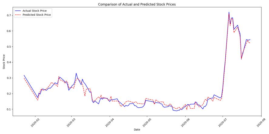
Figure 1: Comparison of Actual and Predicted Stock Prices.

Figure 1 presents that the difference between the output values and the actual values is small, indicating that the constructed BP neural network performs well. The mean square error is 5.61 \( × \) 10-4. Next, for comparison, this research will fit the same data using traditional time series and the Black-Scholes model.

4. Compared with Two Traditional Option Price Prediction Models

4.1. Black-Scholes Model

Black-Scholes Model is an option pricing model derived from the Black-Scholes partial differential equation. The Black-Scholes partial differential equation is a partial differential equation satisfied by option prices. Firstly, it is assumed that the price of the underlying stock satisfies geometric Brownian motion:

\[ dS_{t}=μS_{t}dt+σS_{t}dW_{t} \] (8)

where \( μ \) is the expected rate of return of the corresponding asset, and \( σ \) is the asset volatility. On this basis, assuming that the option price is \( C \) (S,t), then the option price satisfies the partial differential equation:

\[ \frac{∂C}{∂t}+rS_{t}\frac{∂C}{∂S}+\frac{1}{2}σ^{2}S_{t}^{2}\frac{∂^{2}C}{∂S^{2}}=rC \] (9)

where r is the constant interest rate. And from this, the option pricing formula can be derived:

\[ C(S,t)=S_{t}N(d_{1}) - e^{ - r(T - t)}KN(d_{2}) \] (10)

\[ d_{1}=\frac{\ln{(S_{t}/K)+(r - σ^{2}/2)(T - t)}}{σ\sqrt[]{T - t}} \] (11)

\[ d_{2}=d_{1} - σ\sqrt[]{T - t} \] (12)

where K is the option exercise price, and N(·) is the cumulative distribution function of the standard normal distribution.

In this study, the one-year Shanghai Interbank Offered Rate (SHIBOR) is adopted as the risk-free interest rate value. The annualized volatility of Shanghai Stock Exchange 50 ETF in 2020, which is 2.43% (from Wind Information), is taken as the volatility \( σ \) . The contract underlying asset prices from January 23, 2020 to July 18, 2020 are used as the prices in the model for fitting calculation. The obtained fitting mean square error (MSE) is 3.63 \( × \) 10-3.

4.2. Time Series Model

Time series analysis is a statistical method that studies the variation pattern of variables over time based on historical data. It is mainly used to analyze data sequences with time order to reveal characteristics such as trends, seasonality, and periodicity in the data, and for prediction and decision-making.

In time series analysis, commonly used models include auto-regressive model (AR), moving average model (MA), auto-regressive moving average model (ARMA), and auto-regressive integrated moving average model (ARIMA), etc. These models determine the parameters of the model by analyzing the auto-correlation function (ACF) and partial auto-correlation function (PACF) of the data, so as to achieve modeling and prediction of time series.

After conducting the preliminary stationary and white noise tests, this research conducts image analysis of ACF and PACF through Matlab. The results are shown in Figure 2.

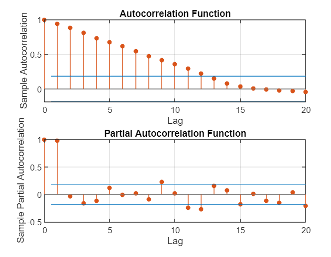
Figure 2: The outcome of ACF and PACF analysis.

As can be seen from Figure 2, the ACF image shows a trailing trend, and the PACF image shows a second-order truncation trend. Therefore, this research finally established an ARIMA(2,2,0) model and obtained Figure 3:

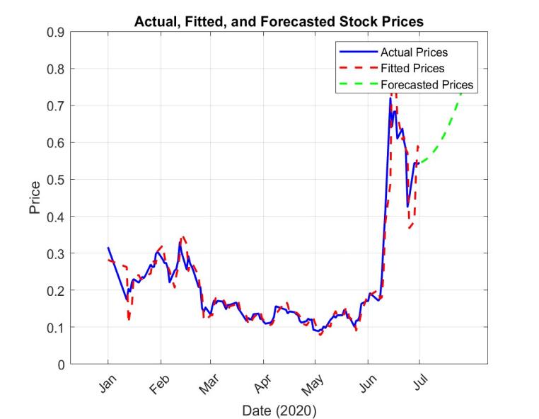
Figure 3: The outcome of the actual, fitted and predicted stock prices.

where its fitting MSE is 2.10 \( × \) 10-3.

4.3. Result Comparison

In summary, this research first summarizes the fitting effects of three different methods. The results are shown in the following table:

Table 2: This fitting results of three models.

As can be seen from Table 2, the fitting mean square error of the BP neural network based on principal component analysis is significantly smaller than that of the other two. It can be seen that its fitting accuracy is relatively the best. At the same time, in order to explore the prediction accuracy of the three models, this article uses three models to predict and analyze the option prices for the trading day data from July 19, 2020 to July 23, 2020 respectively. The obtained results are shown in Table 3:

Table 3: The predicted results of three models.

As can be seen from Table 3, the error between the option calculation price obtained by applying the time series option pricing model and the actual value is relatively large, and its mean square error MSE is7.06 \( × \) 10-2. While the error of the BP neural network algorithm based on principal component analysis is the smallest, and its mean square error MSE is 2.63 \( × \) 10-5. Thus, it can be seen that the BP neural network algorithm based on principal component analysis is feasible for option price prediction, and its prediction accuracy is the highest.

5. Conclusion

This paper is dedicated to conducting research on the prediction accuracy of option prices by using the BP neural network algorithm based on principal component analysis. Through principal component analysis, the input variables in the BP neural network are optimized. This measure can effectively reduce the dimension of input variables, lower the structural complexity of the neural network, and further improve the prediction accuracy of the neural network. The experimental results show that when using the traditional Black-Scholes option pricing method for option price prediction, its prediction accuracy is higher than that of using the time series model for prediction, and the prediction accuracy of the BP neural network algorithm based on principal component analysis is higher than the other two. Therefore, the BP neural network algorithm based on principal component analysis adopted in this paper is feasible in option price prediction research, and the prediction effect of this method is relatively ideal.

References

[1]. Guan Li, Li Yaotang. (2001). Modified Black-Scholes option pricing model. Journal of Yunnan University (Natural Sciences Edition), 23(2), 84-86.
[2]. Zhang Tie. (2000). A novel binomial tree parameter model for option pricing. Systems Engineering Theory and Practice, 20(11), 90-93.
[3]. Li Jiaxin. (2023). Discussion on the Limitations of Option Pricing Models. Economic Perspectives (03), 44-52. doi:10.16528/j.cnki.22-1054/f.202303044.
[4]. Ma Baozhong, Zhen Boqian. (2015). Empirical Analysis of a Gold Futures Price Forecasting Model Based on Time Series Analysis. Business (07), 152.
[5]. Xu Shiyu, Hu Tianhui. (2023). Analysis and Forecasting of the Shanghai Composite Index Based on Time Series. Economic Research Guide (07), 88-90.
[6]. Zhang Lijuan, Zhang Wenyong. (2018). Research on hybrid neural network option pricing based on the Heston model and genetic algorithm optimization. Journal of Management Engineering, 32(3), 8.
[7]. Guan Xueying. (2024). Stock Price Forecasting Based on ARIMA-RNN Hybrid Model. Journal of Harbin University of Commerce (Natural Science Edition) (02), 250-256. doi:10.19492/j.cnki.1672-0946.2024.02.008.
[8]. Qi Taiwei, Yu Wennian. (2024). Multi-Indicator Stock Forecasting Based on LSTM. Computer and Digital Engineering (02), 337-342.
[9]. Liang Yijuan, Xu Chenglong, Ma Junmei.(2018). Principal Component Monte Carlo Acceleration Method for Multi-Factor European Option Pricing. Journal of Southwest University (Natural Science Edition) (01), 88-97. doi:10.13718/j.cnki.xdzk.2018.01.014.
[10]. Chen Jian, Tang Guohao, Yao Jiaquan. (2024). Extraction of Implied Information from Options and Its Impact on the Stock Market: A Machine Learning Perspective. Journal of Econometrics (01), 231-247.
Cite this article
Yao,Y. (2024). Prediction of Option Prices by BP Neural Network Based on Principal Component Analysis. Advances in Economics, Management and Political Sciences,118,289-298.
Data availability
The datasets used and/or analyzed during the current study will be available from the authors upon reasonable request.
Disclaimer/Publisher's Note
The statements, opinions and data contained in all publications are solely those of the individual author(s) and contributor(s) and not of EWA Publishing and/or the editor(s). EWA Publishing and/or the editor(s) disclaim responsibility for any injury to people or property resulting from any ideas, methods, instructions or products referred to in the content.
About volume
Volume title: Proceedings of the 3rd International Conference on Financial Technology and Business Analysis
© 2024 by the author(s). Licensee EWA Publishing, Oxford, UK. This article is an open access article distributed under the terms and
conditions of the Creative Commons Attribution (CC BY) license. Authors who
publish this series agree to the following terms:
1. Authors retain copyright and grant the series right of first publication with the work simultaneously licensed under a Creative Commons
Attribution License that allows others to share the work with an acknowledgment of the work's authorship and initial publication in this
series.
2. Authors are able to enter into separate, additional contractual arrangements for the non-exclusive distribution of the series's published
version of the work (e.g., post it to an institutional repository or publish it in a book), with an acknowledgment of its initial
publication in this series.
3. Authors are permitted and encouraged to post their work online (e.g., in institutional repositories or on their website) prior to and
during the submission process, as it can lead to productive exchanges, as well as earlier and greater citation of published work (See
Open access policy for details).