1. Introduction

The proper pricing of financial derivatives, especially options, is one of the main questions in the finance area. Among the various methods available, In option pricing, Monte Carlo simulation is frequently utilized due to its flexible usage and applicability to various financial models [1]. Monte Carlo Simulation calculates the average payoff of an option by simulating a large set of possible paths of asset price fluctuation. However, a significant limitation of Monte Carlo simulation is the high computational costs, especially when applied to high-dimensional or complex financial derivatives. As the dimensionality of the problem increases, the number of simulations required to achieve accurate pricing increases rapidly, resulting in a large computational overhead [2].

Past studies have tried to solve this problem in multiple ways. The earliest researchers developed Least Squares Monte Carlo (LSMC) Methods, combining simulation with regression techniques to reduce the need for a lot of simulated paths for assets [3]. With advances in machine learning technology, researchers explored the usage of various machine learning techniques (especially neural networks) to improve the efficiency of Monte Carlo simulations. Sebastian Becker et al. use the deep learning method to learn optimal stopping rules from Monte Carlo samples to cut down on the amount of time needed for simulation [4]. Besides, Djagba, et al. discussed the effectiveness of applying methods from machine learning to improve LSMC in option pricing [5]. They discussed multiple machine learning techniques such as RNN, XGBoost, and LSTM model and found that machine learning could effectively reduce the time needed for LSM in American Option pricing.

Based on these past advances, this study explores a hybrid approach to incorporate neural network models into a Monte Carlo simulation framework. This study will use the neural network to regress the intermediate states in the Monte Carlo simulation to predict the subsequent price paths and their corresponding option price. The methods exploit the ability of networks to capture complex, nonlinear dependencies between price paths and returns to provide an effective enhancement methodology for Monte Carlo simulation and its usage in option pricing.

The paper will be organized by the following structure. Initially, there will be a description of the Monte Carlo simulation setup, and then describe in detail the neural network architecture used to predict future simulation paths based on intermediate results. Finally, the study would assess the effectiveness of the hybrid approach by comparing its accuracy and computational efficiency with traditional Monte Carlo simulations.

2. Methodology

2.1. Monte Carlo Simulation Configuration

This study uses a Monte Carlo Simulation framework to do the European option. To make the study focus on investigating the effectiveness of neural networks in predicting subsequent simulations, the study uses a simple European call option. The initial setup for the simulation requires a set of parameters for the options. ​ = 100, strike price K = 100, time to maturity T = 1 year, risk-free interest rate r = 0.05, and volatility σ = 0.2. The simulation involves 100 time steps and generates 100,000 paths to model the stock price evolution over time using geometric Brownian motion (GBM), defined by the stochastic differential equation (SDE):

\( {S_{t}}=r{S_{t}}dt+σ{S_{t}}d{W_{t}} \) (1)

Here in the equation, \( {W_{t}} \) represents a Wiener process (random walk). Each simulated path generates a terminal payoff of \( max({S_{T}}-K,0), \) used to calculate the option's discounted expected payoff. Averaging the discounted payoffs over all simulated pathways yields the final option price. This serves as the baseline for comparison with the neural network-enhanced simulation.

2.2. Neural Network Construction for Path Prediction

The study built a neural network model to predict future simulation paths based on the simulation's intermediate price data to lower the number need of simulated paths while maintaining enough accuracy. The neural network aims to capture the relationship between the intermediate states of a Monte Carlo simulation and the final payoff of the option through a deep learning approach. I used a feedforward neural network with multiple layers and residual blocks. The design of the network follows the deep neural network advanced by He, et al. together with LeCun, et al., where three residual blocks are introduced to enhance the ability of the deep neural network to learn complex, nonlinear relationships without vanishing gradients [6,7].

To prevent model overfitting, the architecture leverages two regularization techniques. First, the Dropout Regularization proposed by Srivastava et al. is used, which is particularly suited for neural networks [8]. This forces the model to develop more resilient, dispersed representations and keeps the network from becoming overly dependent on any one neuron. Second, the L1/L2 weight regularization is used. The L1 regularization adds the weights' absolute values to the loss function, promoting sparsity in the model and resulting in the reduction of many weights to zero, which simplifies the model [9]. On the other hand, L2 regularization adds the weights' squared values, which prevents any single weight from becoming too large, thus distributing learning across all weights [10].

The neural network input consists of the stock prices from the previous 10-time steps (lookback), while the output is the predicted option payoff at maturity. This setup enables the model to effectively learn the nonlinear dynamics between the intermediate price paths and their corresponding payoffs, thus reducing the number of required simulations in subsequent time steps.

The network architecture included:

256 neurons in a fully connected dense layer with ReLU activation.

Three residual blocks, 256 neurons dense layer in each block, batch normalization, L1, L2, and dropout for regularization.

A single-neuron output layer that provides the anticipated payout upon maturity.

2.3. Training and Optimization

Data for training the neural network is derived from the intermediate results of the Monte Carlo simulations. Each simulation path is divided into training samples, where the first 10 time steps serve as input, and the final payoff serves as the label for supervised learning. To train the neural network, split. I used the train_test_split function from the Scikit-learn library to divide the data into training and testing sets with an 80/20 ratio [11].

The training process utilized the Adam optimizer, which combines the benefits of both the AdaGrad and RMSProp algorithms. This enables it to modify the learning rate for every parameter during training by the gradient's first and second moments [12]. Besides, there is also a cyclical learning rate scheduler to dynamically adjust the learning rate during training. To avoid overfitting, early stopping was also added [13]. If the validation loss did not decrease for ten consecutive epochs, the training process would end [14].

Using mean squared error (MSE), we trained the model for 50 epochs with a batch size of 32, which, when used as the loss function to assess how well the model predicts future payoffs, minimizes the discrepancy between the projected and actual payoffs.

2.4. Model Evaluation

By comparing the option prices from the complete Monte Carlo simulation to the neural network's predictions, the effectiveness of the neural network-enhanced simulation is assessed. The primary metric for evaluation is the similarity between the predicted distribution and the original distribution. Besides, the evaluation also includes a direct comparison of the option priced predicted by the reduced path and original price. Additionally, the computational efficiency is assessed by measuring the reduction in simulation time while maintaining an acceptable level of accuracy.

Another European Call Option is used for the evaluation process, and the following specifications are used: Initial stock price \( {S_{0}} \) = 120; Strike price K = 110; Time to maturity = 1.0; Risk-free rate = 0.03; σ = 0.25; Number of time steps = 100; Number of Monte Carlo simulation paths = 10,000

3. Results

To test the ability of the model to reduce the number of simulations used for Monte Carlo simulation on European option pricing, the study employed gradient descent in the number of simulations to test the performance of the completed model trained at every 500 simulations reduction. The simulation starts from 10,000 paths, which is a typical number of Monte Carlo simulations used when doing option pricing.

The study first examines the frequency distribution of the predicted option payoff of the reduced simulation path.

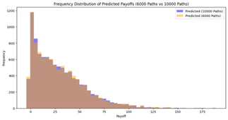
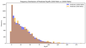
Figure 1: Distribution of Predicted Payoffs of reduced paths compared to 10,000 Paths.

In the frequency table above, the yellow area demonstrates the payoff distribution predicted by the combination of the reduced simulation path and the neural network model, while the blue shaded area demonstrates the original distribution with the 10,000 simulation paths. From Figure 1, As the number of paths decreases (from 9,000 to 2,000), the predicted payoff distributions become progressively sparser and less consistent. For higher path counts, such as 6,000 to 9,000 paths, the predicted distributions closely align with the benchmark distribution (10,000 paths), which clearly shows the stability of the model's predictive capability under reduction.

Performance for moderate path reduction (2,000 – 6,000 paths), the model still shows great stability. Although some minor fluctuations have appeared in the predicted distribution, the overall distribution remains close to the benchmark. This indicates that the model is reaching a boundary point where the model's predictive accuracy starts to significantly degrade.

As seen in the frequency distributions shown in the below 3,000 paths, the predicted distribution starts to diverge from the benchmark in both higher and lower payoff ranges. Thus, Figure 1 shows that around 4,000 to 5,000 paths are a reasonable range for maintaining prediction accuracy while reducing the computational cost

To quantitatively model the similarity of distribution between reduced and original path, the Kolmogorov-Smirnov (KS) Statistics is calculated for each reduced path [15,16].

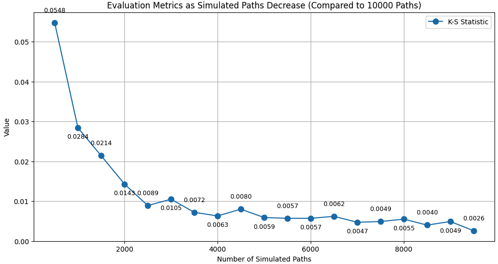
Figure 2: K-S Statistic Evaluation as Simulated Paths Decrease (Compared to 10,000 Paths)

Figure 2 shows the K-S statistic for each distribution. First, even for 2,000 paths, the K-S statistic is close to 0.01, which shows an overall great similarity between the reduced path distribution and the benchmark distribution. However, there is still a clear increasing trend in K-S statistics when reducing number of paths simulated from 9,500 to 500, especially when the number of simulated paths is lower than 4,000. From 4,000 to 9,500 paths, the maximum K-S statistic is 0.01, while this number significantly increases to 0.0143 when the path number is reduced to 2,000. The trend observed in the KS statistic suggests that the similarity of the distribution between the predicted and benchmark option payoffs initially deteriorates as the number of paths decreases. The situation improves significantly as the number of paths increases above 4,000, which demonstrates that maintaining the reduced path at around 4,000 to 5,000 could attain a fair trade-off between computational cost reduction and model performance.

Finally, to more directly look at the predictive accuracy of the model with a reduced path, a final predicted payoff for the call option used in this case is calculated for each reduced simulation path number. The payoff is calculated by taking an average of all the payoffs calculated by the simulated paths and predicted paths by the model.

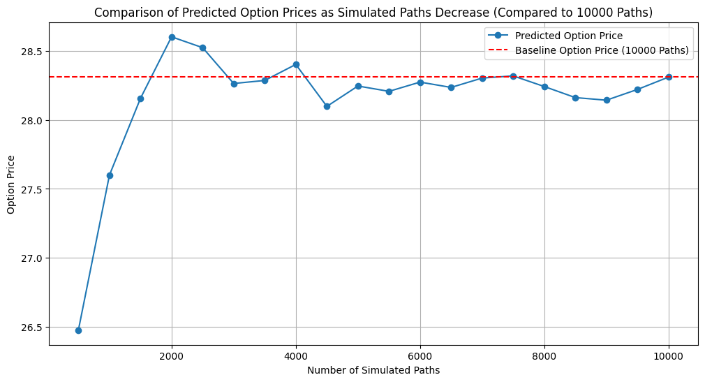
Figure 3: Comparison of Predicted Option Prices as Simulated Paths Decrease

Figure 3 shows a direct comparison between the predicted option price for each reduced number of simulation paths and the baseline option price, which is based on 10,000 Paths. From Figure 3, there is a clear trend that when the number of simulation paths approached 10,000, the predicted option price converged to the baseline value of 28.31. The deviation is small, fluctuating between 28.14 and 28.40. This implies that as the number of pathways grows, the model's ability to represent the underlying distribution of returns improves, leading to predictions that are almost the same as those produced with 10,000 paths. However, when there are fewer than 3,000 simulated pathways, forecasted option prices exhibit significant volatility. This further corroborates our conclusion about the trade-off between reducing the simulation path and maintaining the prediction accuracy. When the path is reduced to 4,000 to 5,000, it is approaching a boundary point for the performance of the model in predicting subsequent paths and making option price predictions.

4. Discussion

This paper has presented an experimental study of employing a neural network to do the regression to the intermediate simulation paths of a Monte Carlo simulation and forecast the future simulation paths, which aims to reduce the number of simulation paths. The experimental findings demonstrate that, when employing Monte Carlo simulation for European option pricing, the approach can dramatically reduce the number of simulations from 10,000 to about 4,000–5,000 without appreciably lowering pricing accuracy. This finding is significant because it effectively reduces the computing cost associated with the huge number of simulations required by typical Monte Carlo methods for pricing high-dimensional or complicated financial derivatives.

The traditional method of Monte Carlo simulation has been broadly used in option pricing, such as European-type options. Boyle asserts that Monte Carlo is a handy and flexible option pricing tool, especially for complex option problems that are difficult to deal with through analytical methods [1]. However, the rise in computing cost of the number of simulation paths is covered by Glasserman [2]. The study introduces neural network regression in the intermediate stage of simulation, which reduces dependence on the increased number of subsequent simulation paths greatly reducing computational complexity and costs. The neural network effectively replaces part of the calculation of subsequent paths by learning and fitting the nonlinear mapping relationships between intermediate simulation states and subsequent simulations. LeCun et al. discuss the strong power of deep neural networks in dealing with nonlinear problems and deep neural networks have the potential to capture complicated nonlinear interactions between inputs and outputs more effectively by expanding the number of network layers [7].

The result of this study ties in with Han, et al. study on the effectiveness of using deep neural networks to capture high-dimensional partial differential equations related to financial option pricing such as the Black–Scholes Equation [17]. In this study, the European option price is calculated by the Black-Scholes Equation [18]. Since the neural network could effectively capture the Black-Scholes Equation, it is effective in predicting subsequent simulations in a Monte Carlo Simulation that is constructed on the Black-Scholes Equation.

However, although this study demonstrates the potential of neural networks in reducing the demand for Monte Carlo simulations, there are still several limitations. First, the predicting accuracy of the neural network relies on full training on the intermediate simulation data, whereas in this study, the training data is based on 10,000 simulation paths. This requires many Monte Carlo simulations in the early stage of training to obtain sufficient training data, which makes the computational overhead of the initial phase of the method still large. This problem is more significant when dealing with more complex options.

Second, despite the strong nonlinear fitting ability of neural networks, its effectiveness in extremely complicated path-dependent alternatives, including American and Asian options, has not yet been thoroughly proven. These options have more dependency on path information, which may require a much more complex structured neural network and more data to capture its features.

5. Conclusion

The study explored the combination of neural network and Monte Carlo Simulation to reduce the number of simulation paths required for accurate option pricing, which reduces the computational cost of using Monte Carlo Simulation in pricing high dimensional financial derivatives. The study reveals that neural networks could effectively reduce simulation paths from 10,000 to around 4,000-5,000 without significantly reducing the prediction accuracy of Monte Carlo simulation. This reduction could greatly reduce the computational cost needed for Monte Carlo Simulation in option pricing. Future studies could focus on exploring more enhancement in the structure of neural networks to boost model performance. For example, the Long Short Term Memory (LSTM) model or VAE performs well in capturing the dynamic feature of time series data. Besides, there could be more attempts to combine predictive models with early stopping techniques that could further optimize computational efficiency.

References

[1]. Boyle, P. P. (1977b). Options: A Monte Carlo approach. Journal of Financial Economics, 4(3), 323–338. https://doi.org/10.1016/0304-405x(77)90005-8
[2]. Glasserman, P. (2003). Monte Carlo methods in financial engineering. Springer.
[3]. Longstaff, F. A., & Schwartz, E. S. (2001). Valuing American options by simulation: a simple least-squares approach. The review of financial studies, 14(1), 113-147.
[4]. Becker, S., Cheridito, P., & Jentzen, A. (2019). Deep optimal stopping. Journal of Machine Learning Research, 20(74), 1-25.
[5]. Djagba, P., & Ndizihiwe, C. (2024). Pricing American Options using Machine Learning Algorithms. arXiv preprint arXiv:2409.03204.
[6]. He, K., Zhang, X., Ren, S., & Sun, J. (2016). Deep residual learning for image recognition. In Proceedings of the IEEE conference on computer vision and pattern recognition (pp. 770-778).
[7]. LeCun, Y., Bengio, Y., & Hinton, G. (2015). Deep learning. Nature, 521(7553), 436–444. https://doi.org/10.1038/nature14539
[8]. Srivastava, N., Hinton, G., Krizhevsky, A., Sutskever, I., & Salakhutdinov, R. (2014). Dropout: a simple way to prevent neural networks from overfitting. The journal of machine learning research, 15(1), 1929-1958.
[9]. Ng, A. Y. (2004, July). Feature selection, L 1 vs. L 2 regularization, and rotational invariance. In Proceedings of the twenty-first international conference on Machine learning (p. 78).
[10]. Krogh, A., & Hertz, J. (1991). A simple weight decay can improve generalization. Advances in neural information processing systems, 4.
[11]. Pedregosa, F., Varoquaux, G., Gramfort, A., Michel, V., Thirion, B., Grisel, O., ... & Duchesnay, É. (2011). Scikit-learn: Machine learning in Python. the Journal of machine Learning research, 12, 2825-2830.
[12]. Kingma, D. P., & Ba, J. (2014). Adam: A Method for Stochastic Optimization. arXiv e-prints, arXiv-1412
[13]. Smith, L. N. (2017, March). Cyclical learning rates for training neural networks. In 2017 IEEE winter conference on applications of computer vision (WACV) (pp. 464-472). IEEE
[14]. Prechelt, L. (2002). Early stopping-but when?. In Neural Networks: Tricks of the trade (pp. 55-69). Berlin, Heidelberg: Springer Berlin Heidelberg.
[15]. An, K. (1933). Sulla determinazione empirica di una legge didistribuzione. Giorn Dell'inst Ital Degli Att, 4, 89-91.
[16]. Smirnov, N. (1948). Table for estimating the goodness of fit of empirical distributions. The annals of mathematical statistics, 19(2), 279-281.
[17]. Han, J., Jentzen, A., & E, W. (2018). Solving high-dimensional partial differential equations using deep learning. Proceedings of the National Academy of Sciences, 115(34), 8505–8510. https://doi.org/10.1073/pnas.1718942115
[18]. Black, F., & Scholes, M. (1973). The Pricing of Options and Corporate Liabilities . Journal of Political Economy, 81(3), 637–654.
Cite this article
Zhang,T. (2024). Neural Network-Enhanced Monte Carlo Simulation for Efficient European Option Pricing. Advances in Economics, Management and Political Sciences,118,205-211.
Data availability
The datasets used and/or analyzed during the current study will be available from the authors upon reasonable request.
Disclaimer/Publisher's Note
The statements, opinions and data contained in all publications are solely those of the individual author(s) and contributor(s) and not of EWA Publishing and/or the editor(s). EWA Publishing and/or the editor(s) disclaim responsibility for any injury to people or property resulting from any ideas, methods, instructions or products referred to in the content.
About volume
Volume title: Proceedings of the 3rd International Conference on Financial Technology and Business Analysis
© 2024 by the author(s). Licensee EWA Publishing, Oxford, UK. This article is an open access article distributed under the terms and
conditions of the Creative Commons Attribution (CC BY) license. Authors who
publish this series agree to the following terms:
1. Authors retain copyright and grant the series right of first publication with the work simultaneously licensed under a Creative Commons
Attribution License that allows others to share the work with an acknowledgment of the work's authorship and initial publication in this
series.
2. Authors are able to enter into separate, additional contractual arrangements for the non-exclusive distribution of the series's published
version of the work (e.g., post it to an institutional repository or publish it in a book), with an acknowledgment of its initial
publication in this series.
3. Authors are permitted and encouraged to post their work online (e.g., in institutional repositories or on their website) prior to and
during the submission process, as it can lead to productive exchanges, as well as earlier and greater citation of published work (See
Open access policy for details).