1. Introduction

Accurately predicting wine quality is essential for the wine industry, as it ensures consistent product standards and supports informed consumer choices. Traditionally, wine quality has been assessed based on subjective characteristics such as flavor, mouthfeel, and aroma, which are inherently linked to its chemical composition. For example, volatile compounds contribute to a wine's aroma, while phenolic compounds influence its flavor [1,2]. This intrinsic relationship between chemical properties and sensory perception allows for an objective and quantitative evaluation of red wine quality, complementing traditional tasting and observation methods and reducing the bias introduced by personal experience and preferences.

With the rise of machine learning, scholars have applied this technology to the prediction of red wine quality. These scholars attempted to compare the predictive performance of various models to select the most applicable model for wine quality assessment. Kumar S and Shaw B, in their studies, added Naive Bayes (NB) and Multilayer Perceptron (MLP) to Random Forest (RF) and Support Vector Machine (SVM), respectively, and both concluded that RF exhibited superior performance. Their conclusion suggested that RF, due to its ability to capture complex non-linear relationships, outperforms other models in scenarios with high data complexity and robustness requirements [3,4]. Building on this, Dahal K R incorporated Gradient Boosting Regressor (GBR) and Artificial Neural Network (ANN) models and found that GBR achieved the highest R value with the lowest Mean Squared Error (MSE) and Mean Absolute Percentage Error (MAPE) [5]. Additionally, Mahima combined RF with K-Nearest Neighbors (KNN) to create a more accurate and dynamic model [6]. On the other hand, researchers have also considered feature selection and analyzed its impact on model performance. Aich S compared the effects of two feature selection algorithms, Principal Component Analysis (PCA) and Recursive Feature Elimination (RFE), on prediction accuracy, and concluded that the feature combination under RFE can achieve better prediction accuracy [7]. Bhardwaj P, Jain K, and Yogesh Gupta found that feature selection significantly affects the accuracy of non-ensemble models such as RF, SVM, and ANN, but has little impact on boosting models like Adaptive Boosting (AdaBoost) and Extreme Gradient Boosting (XGBoost) [8-10].

To enhance wine quality prediction models, this study refines previous approaches by constructing and analyzing new features using the Wine Quality dataset. It identifies the most impactful features and applies them to the RF model, which shows superior performance and stability compared to models with original features. Key features such as alcohol, free sulfur dioxide, and sulfates significantly improve prediction accuracy. However, caution is advised as creating new features can sometimes negatively affect the model. This work highlights the importance of effective feature engineering in developing robust prediction models.

2. Methodology

2.1. Dataset Description and Preprocessing

This study uses data from the Wine Quality dataset, published on June 10, 2009, in the UCI Machine Learning Repository which includes 1,599 red wine samples, with no missing values [11]. It contains 11 floating point features describing the physical and chemical properties of wine, and the target variable quality is of integer type ranging from 3 to 8. Table 1 shows some examples.

Table 1: Dataset examples.

To address issues such as outliers, skewed distributions, varying feature ranges, and class imbalance, several preprocessing steps were undertaken. Outliers were managed with the Interquartile Range (IQR) method and Fissurization. Left-skewed features were adjusted using Logarithmic Transformation. Two additional features, Total Acidity and Sulfur Dioxide Ratio, were created to improve model performance. Standardization was applied to ensure uniformity across features with different ranges. Finally, Stratified Shuffle Split was employed to maintain consistent class proportions in the training and testing sets.

2.2. Proposed Approach

This study focuses on optimizing wine quality prediction through feature selection and model enhancement. The primary objective is to identify the optimal feature combinations and models to improve predictions for red wine quality. To achieve this, a comprehensive five-dimensional evaluation framework was developed, assessing models based on accuracy, precision, recall, F1 score, and Area Under the Receiver Operating Characteristic Curve (AUC-ROC). The models compared include RF, Logistic Regression (LR), KNN, SVM, and NB, to identify the most effective predictor for wine quality. Prior to model training and feature selection, the data was preprocessed, as detailed in Chapter 2.1. RFE was then employed to rank features by their importance. Features were incrementally added to model training and evaluation. A graph illustrating changes in model performance with varying numbers of features was created. Unimportant and redundant features were removed, and the remaining features were used to form new feature combinations.

Subsequently, the best model is selected from the five models based on the performance of the above five dimensions. The newly selected feature combinations were applied to the best-performing model, and hyperparameters were tuned using grid search. The optimized model was tested and validated for stability and generalization using cross-validation. Additionally, the importance of each feature was evaluated and ranked. The impact of feature selection on prediction accuracy was compared before and after feature selection, as depicted in Figure 1.

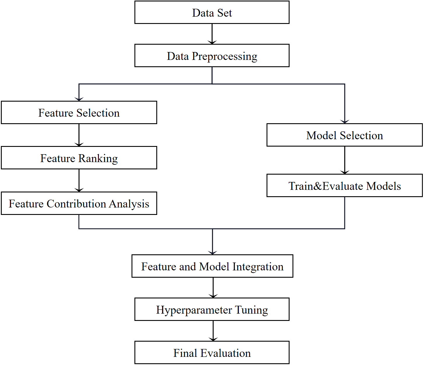
Figure 1: Architectural diagram.

2.2.1. Random Forest (RF)

RF utilizes a technique called bagging, which uses a bootstrap procedure to generate subsamples from the original dataset and independently distributes these subsamples on different subsets. Subsequently, a decision tree model is trained for each subsample. In the classification problem, RF votes based on the prediction results of all decision trees. In the regression problem, the prediction results are averaged to obtain the final prediction result. This method avoids the learning of all samples and all features for each tree, thereby effectively reducing the overfitting phenomenon of a single model. It can also give full play to the advantages of different models through parallel training, thereby significantly improving the overall prediction performance. Unlike boosting, each model of RF is trained independently and in parallel. This diverse ensemble learning strategy enables RF to perform well in various prediction tasks.

2.2.2. Logistic Regression (LR)

LR specialize in solve classification problems, especially for binary classification problems. Its essence is a discriminant model based on conditional probability. Its principle is to combine the linear model of the model with the Sigmoid function. The Sigmoid function maps the linear model output to a probability value between 0 and 1, thereby indicating the probability that the sample belongs to a certain category or the positive or negative classification.

\( f(z)=\frac{1}{1+{e^{-z}}}\ \ \ (1) \)

where z is the output of the linear model.

Secondly, the gradient descent method or other optimization algorithms are used to reduce the prediction error by minimizing the log-likelihood loss function (Log-Loss). Finally, the trained model is used to classify and predict new samples, and the category label is determined based on the predicted probability value. However, LR is weak in dealing with nonlinear relationships. When dealing with nonlinear problems, its modeling ability can be improved by introducing nonlinear extensions and other methods.

2.2.3. K-Nearest Neighbors (KNN)

KNN is a prediction method that does not require the construction of a mathematical model. In the prediction stage, KNN classifies the K samples with the most similar features between the training data set and the samples to be classified into the same category. This is due to KNN algorithm believes that samples with the same category are also similar in feature space. Usually, different distance measurement tools such as Euclidean distance can be used for example measurement between the training set and the samples to be classified. On this basis, the model selects the model closest to the K example samples and votes to confirm the category based on its category. It is worth noting that smaller neighbor samples may cause the model to be sensitive to noise, while larger neighbor samples may cause data details to be ignored, so the selection of K value needs to be cautious.

2.2.4. Support Vector Machine (SVM)

SVM’s main idea is to perform classification or regression by finding an optimal hyperplane or linear decision boundary in the feature space. Specifically, find the sample points closest to the decision boundary and use these points to find a decision surface so that there is as large a gap as possible between the two categories, that is, minimize the distance between all data points and the decision boundary. Ideally, SVM will find a hyperplane that can classify correctly, which is called a hard margin. However, contrary to the fact that data is linearly separable, in reality, data often contains all kinds of noise and errors. Therefore, soft margins are used. Soft-margin SVM introduces slack variables and minimizes the product of the slack variables and the penalty factor to reduce the number of misclassified samples. For linearly inseparable data, SVM can employ various kernel functions tailored to the specific characteristics of the data to map samples into a higher-dimensional feature space. This approach facilitates linear separability within this new space, avoiding the computational complexity associated with directly working in high-dimensional feature spaces.

2.2.5. Naive Bayes (NB)

As an algorithm based on Bayes' theorem, NB also requires that each feature obeys the conditional independence assumption. The essence of this algorithm is that the posterior probability of a given sample in each category represents the possibility of it in the category to which it belongs, so the algorithm uses the category with the maximum posterior probability as the prediction result.

Bayes' theorem expresses the probability of a new sample in its category by describing the relationship between conditional probabilities. The conditional independence assumption of features assumes that under the condition of a given category, the features are independent of each other, which simplifies the calculation process. However, in reality, features are not usually independent of each other. On the other hand, due to the premise of feature independence, the correlation between some features is difficult to capture. Such characteristics may reduce its prediction accuracy.

3. Result and Discussion

This study analyzes performance of model change with number of features and screens out new feature combinations. On the other hand, the best applicable model is selected through model performance evaluation. After hyperparameter tuning, a final test using cross validation was performed, and the model performance, generalization ability, and stability were evaluated. The effect of feature selection on model performance will be further analyzed, and the importance of each feature in the new combination will be explored.

3.1. Impact of Features on Model Performance

Figure 2 shows the change of prediction accuracy of each model as the number of features increases. The first two features contribute the most to the model, and the first-ranked feature, Alcohol, alone can bring at least 50% accuracy to the model. When there are 3 features, the accuracy of most models tends to stabilize. From the analysis of the negative impact of model prediction, the addition of the fourth feature density leads to a significant decrease in the prediction accuracy of models other than RF. The seventh and ninth features, namely the ratio of chloride to sulfur dioxide, also have a negative impact on models other than LR. The last three features have almost no impact on the model accuracy. The same trend is also shown in Precision, Recall, and F1-score.

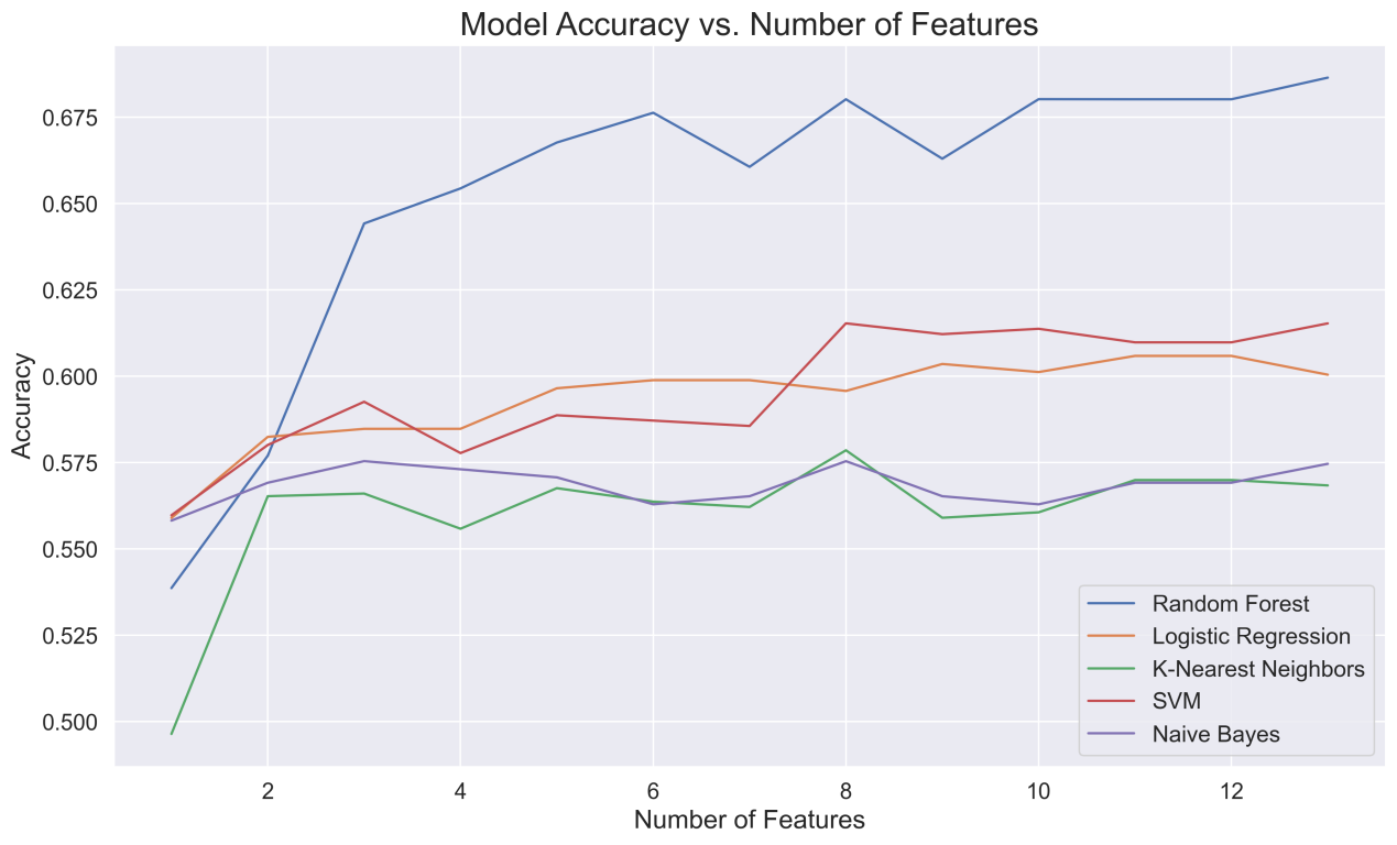
Figure 2: Model accuracy vs features.

The features in Figure 3 are slightly different from those in the previous figure. The fifth and sixth feature densities and total acidity are the reasons for the decrease in the AUC-ROC values of each model, while these features have little effect on the accuracy of the previous figure.

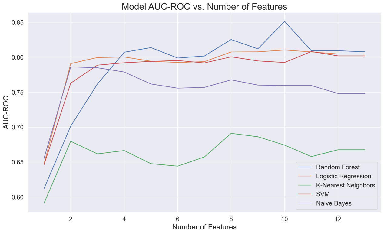
Figure 3: Model AUC-ROC vs features.

In summary, alcohol content and volatile acidity have the most significant effect on improving model performance. More features will only improve the model to a limited extent, and the addition of specific features does not always have a positive impact on the predictive ability of the model. This may be due to the redundancy of features or the influence of irrelevant features. In the 3.3 new feature combination and optimal model retraining stage, the new feature combination uses the remaining features after deleting the above-mentioned 6 features that have a negative impact on the model and the features at the bottom of the ranking. The new feature combination includes alcohol, sulphates, volatile acidity, fixed acidity, total sulfur dioxide, citric acid and ph.

3.2. Model Selection and Evaluation

Figure 4 shows the performance indicators of each model. As can be seen from the figure, the RF model has obvious advantages over other models in the first four dimensions, and each evaluation index is ahead by about 0.05, especially in the two indicators of Accuracy and Recall. The AUC-ROC index of the five models is relatively small. Except for the weak performance of the KNN and NB models, the performance level of LR and SVM is also close to RF, reaching 0.80, which can effectively distinguish between positive and negative classes.

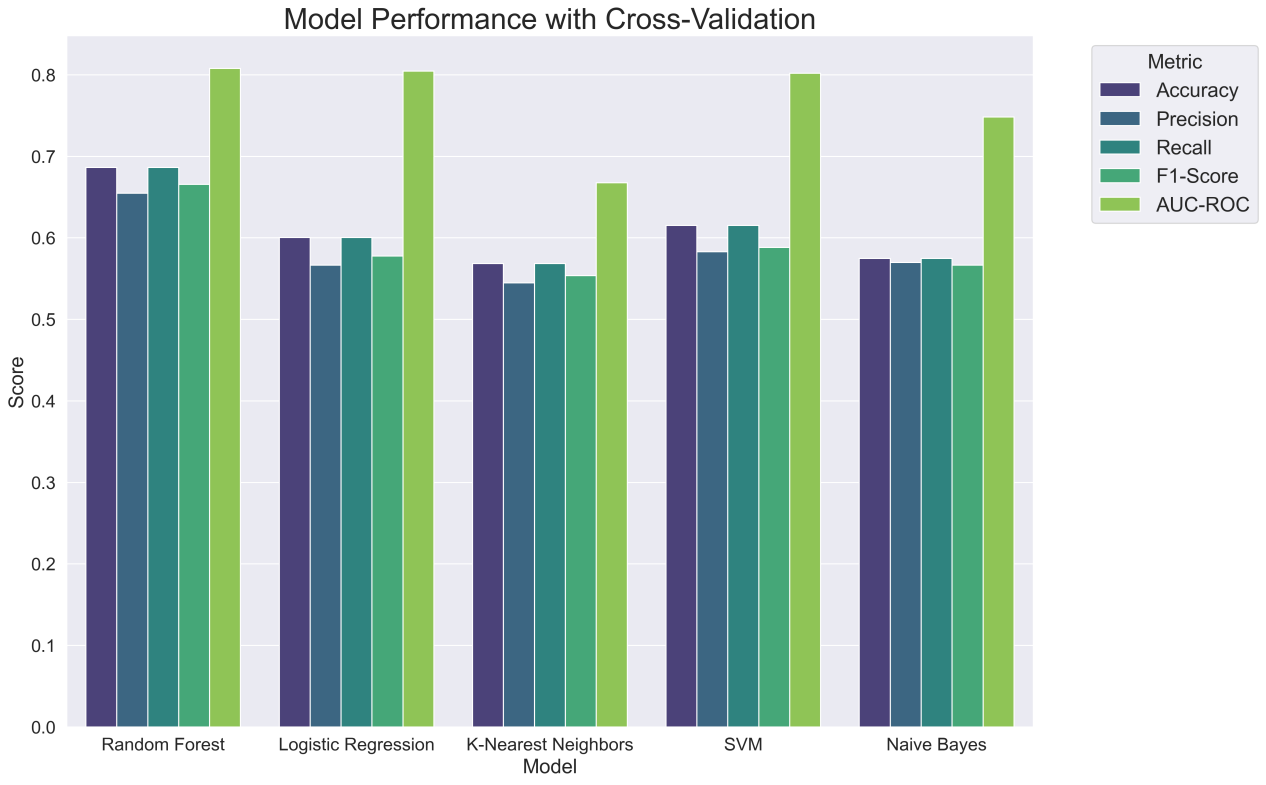
Figure 4: Model performance with cross-validation.

Based on the five indicators, it can be seen that the RF model has the best performance and is more suitable for red wine quality prediction.

3.3. Final Assessment

In this stage, the new feature combination obtained in Section 3.1 and the optimal performance model obtained in Section 3.2 are used for hyperparameter tuning to study the model performance, performance improvement brought by feature selection, and feature importance.

3.3.1. Model Performance Improvement Analysis

The evaluation results of substituting the new feature combination into RF are shown in Figure 5. The new model performs stably in all three datasets, with the performance difference not exceeding 0.009. This shows that the new model has good generalization ability and stability.

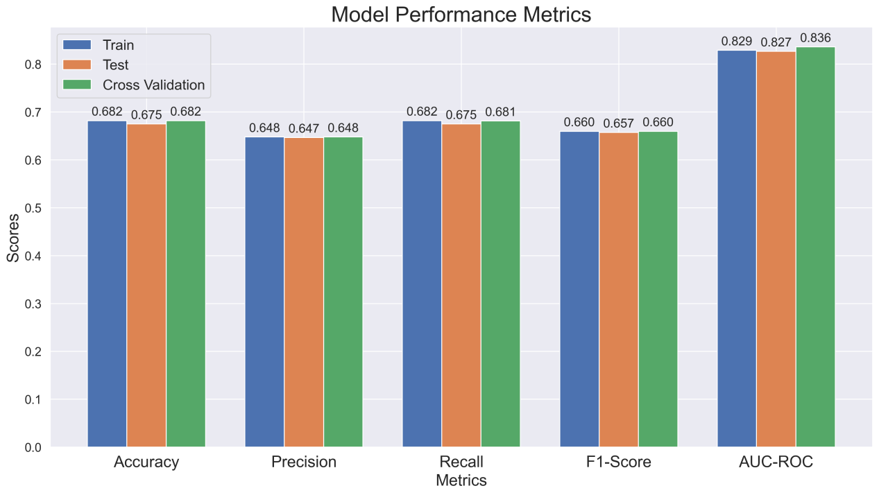
Figure 5: Model performance metrics.

Figure 6 shows the performance improvement brought by feature selection on the training set, test set and CV in various evaluation dimensions. The test set and cross-validation showed an improvement of about 0.08 except for AUC-ROC, among which the improvement of cross-validation in AUC-ROC was the most prominent, reaching 0.175. This shows that feature selection can effectively avoid the influence of noise features on the model while reducing the complexity of the model.

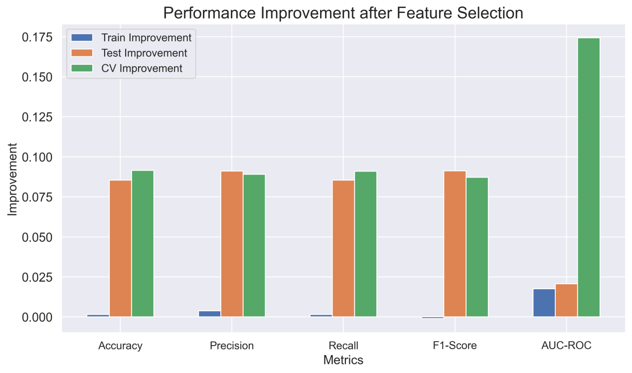
Figure 6: Performance improvement after feature selection.

3.3.2. Feature Importance Analysis

Using the built-in feature importance of the RF model, this study found that the feature importance decreased in three gradients. Among them, alcohol content is the most critical indicator for red wine prediction, with an importance of 0.22. Sulfate, volatile acidity, and citric acid are the second gradient features, and their importance is also close to 0.15. These features are likely to effectively capture information complementary to alcohol content. The third gradient is fixed acidity, free sulfur dioxide, and pH value, which have an importance of 0.11, but still play a certain role in the model.

4. Conclusion

This study builds on previous research by enhancing wine quality prediction through improved model selection and feature analysis. A comprehensive feature selection system was proposed, involving the creation of new features, evaluating their contributions, and ranking their importance. RFE was used to rank features, which were then applied to various machine learning models—RF, LR, KNN, SVM and NB. The study demonstrated that the RF model with feature selection surpasses models using original features in terms of generalization and stability. Feature selection effectively reduces noise and redundant features, lowers model complexity, and enhances prediction accuracy. Key features such as alcohol, free sulfur dioxide, and sulfates significantly improve model performance, aligning with sensory observations where alcohol content, for example, impacts the wine’s body, taste, and aroma. However, constructing new features does not always enhance performance. For instance, the "total acidity" feature may lead to information loss, and the "Sulfur Dioxide Ratio" may complicate the model without reflecting sulfur dioxide's true impact. Future research will address class imbalance and explore sampling techniques to further optimize feature selection and prediction accuracy.

References

[1]. Cortez, P., Cerdeira, A., Almeida, F., et al. (2009) Modeling wine preferences by data mining from physicochemical properties[J]. Decision support systems, 47(4), 547-553.
[2]. Waterhouse, A.L., Frost, S., Ugliano, M., et al. (2016) Sulfur dioxide–oxygen consumption ratio reveals differences in bottled wine oxidation[J]. American Journal of Enology and Viticulture, 67(4), 449-459.
[3]. Kumar, S., Agrawal, K., Mandan, N. (2020) Red wine quality prediction using machine learning techniques. 2020 International Conference on Computer Communication and Informatics, 1-6
[4]. Shaw, B., Suman, A.K., Chakraborty, B. (2020) Wine quality analysis using machine learning. Emerging technology in modelling and graphics: proceedings of IEM graph, 239-247.
[5]. Dahal, K.R., Dahal, J.N., Banjade, H., et al. (2021) Prediction of wine quality using machine learning algorithms. Open Journal of Statistics, 11(2), 278-289.
[6]. Mahima, Gupta, U., Patidar, Y., et al. (2020) Wine quality analysis using machine learning algorithms. Micro-Electronics and Telecommunication Engineering, 11-18.
[7]. Aich, S., Al-Absi, A.A., Hui, K.L., et al. (2018) A classification approach with different feature sets to predict the quality of different types of wine using machine learning techniques. 2018 20th International conference on advanced communication technology, 139-143.
[8]. Bhardwaj, P., Tiwari, P., Olejar, Jr.K., et al. (2022) A machine learning application in wine quality prediction. Machine Learning with Applications, 8, 100261.
[9]. Jain, K., Kaushik, K., Gupta, S.K., et al. (2023) Machine learning-based predictive modelling for the enhancement of wine quality. Scientific Reports, 13(1), 17042.
[10]. Gupta, Y. (2018) Selection of important features and predicting wine quality using machine learning techniques. Procedia Computer Science, 125: 305-312.
[11]. Vapnik, V. (2013) The nature of statistical learning theory. Springer science & business media, 3, 125.
Cite this article
Xu,B. (2024). Optimizing Red Wine Quality Prediction: The Impact of Feature Selection and Model Evaluation. Advances in Economics, Management and Political Sciences,139,1-8.
Data availability
The datasets used and/or analyzed during the current study will be available from the authors upon reasonable request.
Disclaimer/Publisher's Note
The statements, opinions and data contained in all publications are solely those of the individual author(s) and contributor(s) and not of EWA Publishing and/or the editor(s). EWA Publishing and/or the editor(s) disclaim responsibility for any injury to people or property resulting from any ideas, methods, instructions or products referred to in the content.
About volume
Volume title: Proceedings of the 3rd International Conference on Financial Technology and Business Analysis
© 2024 by the author(s). Licensee EWA Publishing, Oxford, UK. This article is an open access article distributed under the terms and
conditions of the Creative Commons Attribution (CC BY) license. Authors who
publish this series agree to the following terms:
1. Authors retain copyright and grant the series right of first publication with the work simultaneously licensed under a Creative Commons
Attribution License that allows others to share the work with an acknowledgment of the work's authorship and initial publication in this
series.
2. Authors are able to enter into separate, additional contractual arrangements for the non-exclusive distribution of the series's published
version of the work (e.g., post it to an institutional repository or publish it in a book), with an acknowledgment of its initial
publication in this series.
3. Authors are permitted and encouraged to post their work online (e.g., in institutional repositories or on their website) prior to and
during the submission process, as it can lead to productive exchanges, as well as earlier and greater citation of published work (See
Open access policy for details).