1. Introduction

1.1. Background

It’s acknowledged that the value of financial derivatives is obtained from the underlying assets. Hence, the value of derivatives can be calculated theoretically by analyzing the characteristics of underlying assets. Therefore, accurate option pricing is essential for financial investors to construct investment portfolios. Options allow investors to hedge risks and enhance portfolio returns without owning the underlying assets.

The Nasdaq Index, S&P 500 Index, and Dow Jones Industrial Average (DJIA) are the three most representative and influential indices in the United States. They can reflect the market's confidence in the macro-economy and various industries and influence investors' investment decisions. The three major indices have different focuses and do not use the same index measurement method. The NASDAQ-100 Index includes the 100 largest non-financial companies listed on the NASDAQ, focusing on the technology sector. The S&P 500 Index includes 500 top U.S. companies across various industries, while the DJIA tracks 30 significant companies, emphasizing industrial enterprises. These indices are commonly used as underlying assets in numerous daily-traded options contracts.

The Black-Scholes model is a widely used method for option pricing, which can provide a solution and offer high efficiency to market trends and daily trading. However, the BS model's assumption of constant volatility has always been criticized for its lack of realism, as realistic market volatility is often dynamic and constantly changing, potentially leading to inaccuracies in option pricing.

1.2. Related Research

1.2.1. Research on the BS Model

Option pricing is critical for the financial industry as it helps determine the fair value of options, optimizes risk management, and supports investment decisions, thereby maintaining the overall robustness of financial markets and providing profit for the whole industry. The Black-Scholes model offers a theoretical foundation for option pricing in financial markets, introducing the no-arbitrage principle and helping market participants evaluate the theoretical value of options, promoting fairness and consistency in market pricing. Initially developed by Fischer Black and Myron Scholes, the BSM model posited that a theoretical option pricing formula could be derived by constructing a trading strategy that includes long/short options and their underlying assets, applicable not only to corporate liabilities but also to a broad range of underlying assets including stock indices [1]. Tong noted that the BSM model, grounded in stochastic processes and calculus, provides a mathematically derived closed-form solution for option pricing by constructing arbitrage strategies to eliminate the unpredictability of stochastic Brownian motion [2]. After creating the trading portfolio, many researchers noted that the constant volatility assumption in the BSM model does not hold in fundamental markets where volatility is constantly changing. Bayraktar and Poor expanded upon previous research by exploring stochastic volatility models modulated by fractional Brownian motion or its time changes [3]. They developed an arbitrage strategy suitable for a modified Black-Scholes model driven by fractional Brownian motion, especially when dealing with stochastic volatility. In their pursuit of methods to enhance option pricing accuracy within the BSM model, Lahouel and Hellara utilized newly modified GARCH processes to improve the constant fluctuations in the BS model to conditional volatility calculated based on historical volatility and data, using real data from the CAC 40 index to study the performance of various models in terms of maturity and moneyness [4]. They concluded that the GARCH approach was the most accurate method for providing more precise option pricing for the BSM model.

1.2.2. Research on the GARCH Model

The BSM model initially assumed that volatility is constant. However, in financial markets, the volatility of the underlying assets fluctuates over time, so this assumption does not match the actual situation. Engle proposed the ARCH model to address this limitation to model volatility in time series data [5]. The ARCH model posits that current volatility depends not only on the mean of historical data but also on historical volatility, and it also predicts the variance of error terms through the square of past error terms. This approach is deemed suitable for volatility modeling in financial markets since it typically exhibits clustering effects. However, the ARCH model often requires many lag terms to capture volatility characteristics in the data, which increases complexity and might lead to overfitting problems. To deal with these problems, the GARCH model emerged as the times required, which improves and expands the ARCH model and enhances the model’s descriptive power. Duan extended the model by introducing a corresponding delta formula and demonstrated that under certain combinations of preference and distribution assumptions, the GARCH option pricing model can effectively reflect changes in the conditional volatility of the underlying asset [6]. Bhat and Arekar compared the performance of the BSM model and Duan’s NGARCH option pricing model in USD-INR exchange-traded currency options, concluding that the GARCH model performed more accurately during periods of market volatility, particularly during periods of significant market turbulence [7]. Furthermore, Adesi proposed a new option pricing method based on the GARCH model using extensive empirical analysis of S&P 500 index options [8]. This enhanced the model's ability to adapt to market prices under incomplete market conditions.

1.2.3. Research on Stock Index

The Nasdaq Index, S&P 500 Index, and Dow Jones Industrial Index are three major indices in the U.S. financial market, each renowned for its unique calculation method, industry focus, and the specific market segments they reflect. These indices are also considered critical underlying assets in options trading. The Nasdaq-100 Index primarily focuses on the performance of large U.S. technology companies. Thomas pointed out that companies with a high proportion of critical patents are more likely to create breakthroughs in the field of technology, and these companies usually perform well in the Nasdaq capital market [9]. In contrast, Rahman’s research focuses on the Dow Jones Industrial Average(DJIA), emphasizing that the performance of DIJA largely depends on the performance of American industrial giants [10]. He found that the volatility of the DJIA is more dependent on historical data and that futures and futures options trading have not caused significant structural changes in the conditional volatility of its component stocks. On the other hand, the S&P 500 Index is regarded as a representative indicator of the performance of the overall U.S. economy and multiple industries due to its broad industry coverage. By analyzing the distinct characteristics and focuses of these three indices, studying the impact of the refined GARCH model on the accuracy of the BS model in pricing options on these indices will provide researchers and traders with more profound and more valuable insights, especially in evaluating the application effect of the GARCH model in different industries. More specifically, this will further help determine which industries are most suitable for using the improved GARCH model to improve the accuracy of option pricing.

1.3. Objective

The purpose of this study is to improve the precision of option pricing by incorporating the GARCH model into the BS model, taking advantage of the GARCH model’s ability to capture the dynamic changes in market volatility, and evaluating the performance of the GARCH-enhanced BS model in different industries. The subjects of this study are options related to the three major US stock indices: the NASDAQ 100, the S&P 500, and the Dow Jones Industrial Average (DJIA). Through an in-depth analysis of the characteristics of these index constituent stocks, the research will reveal the effect of the GARCH model in improving the accuracy of BS model option pricing in different industry sectors. Ultimately, this study will provide specific insights into applying the GARCH model to enhance the BS model in various industries, providing a reference and decision-making basis for financial institutions and traders when choosing the most appropriate option pricing method.

2. Data and Method

The sample for this study consists of the S&P 500, NASDAQ-100, and the Dow Jones Industrial Average ETF (DIA). The NASDAQ-100 Index was selected over the NASDAQ Composite because its number of constituent companies aligns more closely with the S&P 500 and the Dow Jones Industrial Average. Furthermore, the NASDAQ-100's emphasis on the technology sector is valuable for this study’s examination of option pricing across various industries. The choice of DIA is due to its similar sector weighting as the Dow Jones Industrial Average but with a higher daily trading volume, enhancing the robustness of the analysis.

2.1. Data Description

This study aims to empirically analyze U.S. stock index options to investigate the effectiveness of the GARCH model in enhancing the BSM model's option pricing capabilities and to compare its optimization effects across different industries. Therefore, the study has collected trend data spanning five years, from August 13, 2019, to August 13, 2024, for the NASDAQ-100 Index, S&P 500 Index, and SPDR Dow Jones Industrial Average ETF Trust. Before implementing the BSM model and GARCH optimization, this study will analyze the data for these three indices to ensure their characteristics are suitable for BSM pricing and GARCH model enhancements.

In this study, the log return distributions and autocorrelation plots for these three assets will be used to analyze the overall data distribution.

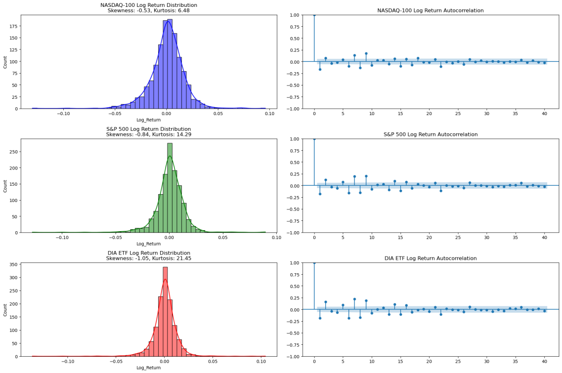
Figure 1: The log return distributions and autocorrelation plots

Figure 1 shows that the logarithmic returns of the Nasdaq 100 are approximately normally distributed but have significant leptokurtic (fat-tailed) characteristics, indicating that extreme returns occur more frequently than normal Distribution predictions. Such fat-tailed phenomena are commonly observed in financial markets, particularly in indices dominated by high-volatility tech stocks. Similarly, the S&P 500 log return distribution also approximates normal but with comparable leptokurtic features. Given its broader market coverage across various industries, the overall volatility of the S&P 500 typically remains lower than that of the NASDAQ-100, yet it still exhibits notable volatility clustering. Meanwhile, the Dow Jones Industrial Average also shows fat-tailed characteristics, albeit to a lesser extent. This may be attributed to the index comprising mature industrial and consumer goods firms, which inherently exhibit lower volatility. Despite this, the potential for extreme outcomes remains even in an index with lower volatility.

Based on the log return distribution charts for the three major indices, this study found that the logarithmic return distributions of each index exhibit the typical characteristics of a normal distribution found in financial time series. However, there is also a prominent presence of leptokurtosis or "fat tails.", which indicates a higher probability of extreme positive and negative returns, suggesting more significant market risks than those projected by a standard normal distribution.

From the autocorrelation distribution charts for three indices, log returns exhibit little significant autocorrelation across most lags. This independence of market-day price changes is consistent with the efficient market hypothesis. Nevertheless, there is often an observable volatility clustering during periods of high market volatility. This phenomenon can lead to autocorrelation at certain lags, particularly over extended periods. Such patterns underscore the applicability of the GARCH model, which is particularly adept at modeling and forecasting time-varying volatility, making it a fundamental tool for understanding and mitigating risks in financial markets. This study provides a compelling argument for using GARCH models to enhance the robustness of financial analytics, especially in turbulent market conditions.

2.2. Calculation Method

2.2.1. BSM Model

The Black-Scholes-Merton (BSM) model provides a mathematical method to price European call options. The BS formula for calculating the value of the option on a non-dividend underlying stock is as follows:

\( C_{0}=S_{0}N(d_{1}) - Ke^{ - rT}N(d_{2})\ \ \ (1) \)

\( N(x)≔P[Z≤X]=\frac{1}{\sqrt[]{2π}} \in t\ _{ - ∞}^{x} e^{ - \frac{y^{2}}{2}dy}\ \ \ (2) \)

\( d_{1}=\frac{1}{σ\sqrt[]{T - t}}[\log{(\frac{s(t)}{K})}+(r+\frac{σ^{2}}{2})(T - t)]\ \ \ (3) \)

\( d_{2}=\frac{1}{σ\sqrt[]{T - t}}[\log{(\frac{S(t)}{K})}+(r - \frac{σ^{2}}{2})(T - t)]=d_{1} - σ\sqrt[]{T - t}\ \ \ (4) \)

For a European put option, the formula is slightly modified:

\( P=Ke^{ - rT}N( - d_{2}) - S_{0}N( - d_{1})\ \ \ (5) \)

C0 is the call option price, S0 is the asset's current price, K is the option's strike price, r is the risk-free interest rate, T is the option's time to expiration, and σ is the volatility of the stock’s returns.

2.2.2. GARCH model

The GARCH model is a significant extension of the ARCH model, providing an advanced method for analyzing the volatility in time series data. The GARCH (1,1) model, the most used variant, is mathematically expressed as:

\( σ^{2}=ω+αϵ_{t - 1}^{2}+βσ_{t - 1}^{2}\ \ \ (6) \)

Where \( σ^{2} \) represents the conditional volatility at time t, calculated based on all available historical data, including the past volatility and stock prices, forecasting the volatility of returns at time t; \( ϵ_{t - 1}^{2} \) is the squared residual at time t-1, reflecting the deviation between actual and predicted returns; ω,αandβare model parameters, typically estimated through maximum likelihood estimation. These parameters capture the volatility of asset returns and reflect the dynamic self-adjusting capability of volatility.

The core advantage of the GARCH model lies in its efficient capture of "volatility clustering"—the situation in which volatility tends to be concentrated within specific periods rather than evenly distributed. The GARCH model offers an analytical framework that more closely aligns with the actual behavior of financial markets. It dynamically adjusts volatility forecasts, aligning more closely with the characteristic variability of stock, index, or other asset prices over time.

3. Result

This study first calculates the option pricing of the three major stock indices using the BS model and Monte Carlo simulations. Then, this study uses the GARCH model to estimate the conditional volatility to enhance the accuracy of volatility within the BS model. Finally, the RMSE evaluation of the option prices obtained by the two methods is conducted to demonstrate whether GARCH optimization significantly affects the accuracy of option pricing. The Monte Carlo method is used in this study to improve option price estimation.

3.1. Original BS Model in Mont-Carlo Simulation

3.1.1. Option Pricing in SPX Index

For the SPX index simulation, this study selected a European call option with a maturity date of January 17, 2025, as the subject of analysis (Figure 2). The risk-free rate used in the simulation was the 10-year U.S. Treasury bond yield at the time of the study (the same risk-free rate was applied in the option pricing analysis for both NDX and DIA).

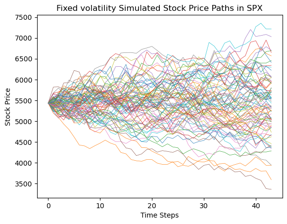
Figure 2: Fixed volatility simulated stock price paths in SPX

Based on the BS model and Monte Carlo simulations, this study conducted 10,000 simulations on the SPX index. The final option prices under different strike prices are calculated in Table 1.

Table 1: SPX Option Pricing Across Varying Strike Prices

3.1.2. Option Pricing in NDX Index

In the simulation of the NDX index, to maintain consistency in the trading times of the options across the three indices, this study selected a European call option with a maturity date of January 17, 2025, as the subject of analysis. The specific simulation results and the prices under different strike prices are shown in Figure 3 and Table 2.

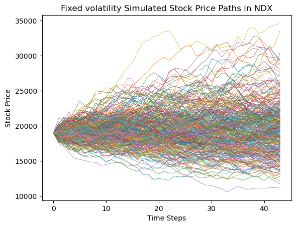
Figure 3: Fixed volatility simulated stock price paths in NDX

Table 2: NDX Option Pricing Across Varying Strike Prices

3.1.3. Option Pricing in DIA Index

In the simulation of the DIA index, to maintain consistency in the trading times of the options across the three indices, this study selected a European call option with a maturity date of January 17, 2025, as the subject of analysis. The specific simulation results and the prices under different strike prices are shown in the Figure 4 and Table 3.

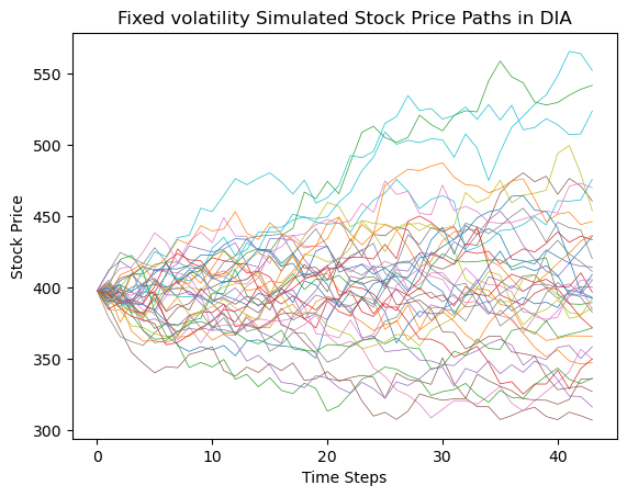
Figure 4: Fixed volatility simulated stock price paths in DIA

Table 3: DIA Option Pricing Across Varying Strike Prices

3.2. GARCH Integration in Mont-Carlo Simulation

After confirming that the options for all three indices in this study (SPX, NDX, and DIA) are suitable for fitting using the GARCH model, the conditional volatility for SPX, NDX, and DIA was first calculated. Figure 5, Figure 6 and Figure 7 illustrate the conditional volatility trends for the three indices: SPX, NDX, and DIA.

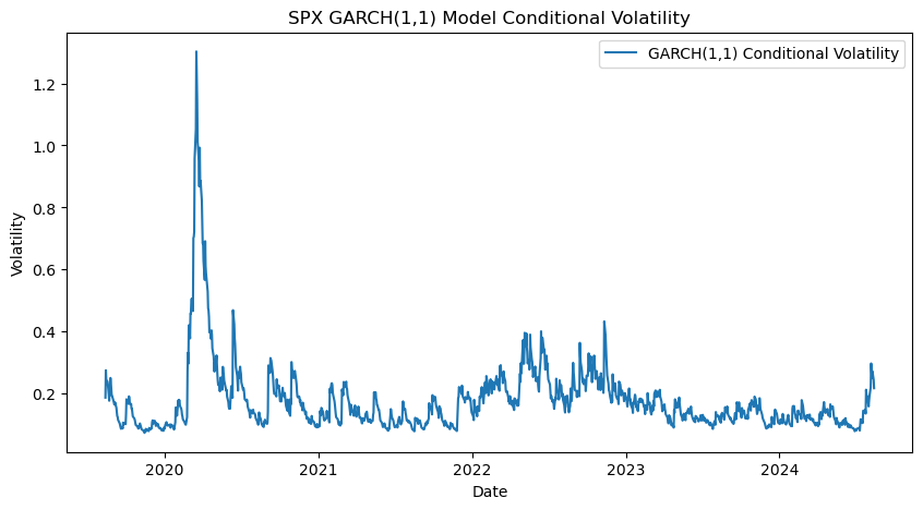
Figure 5: SPX Conditional Volatility Based on the GARCH(1,1) Model

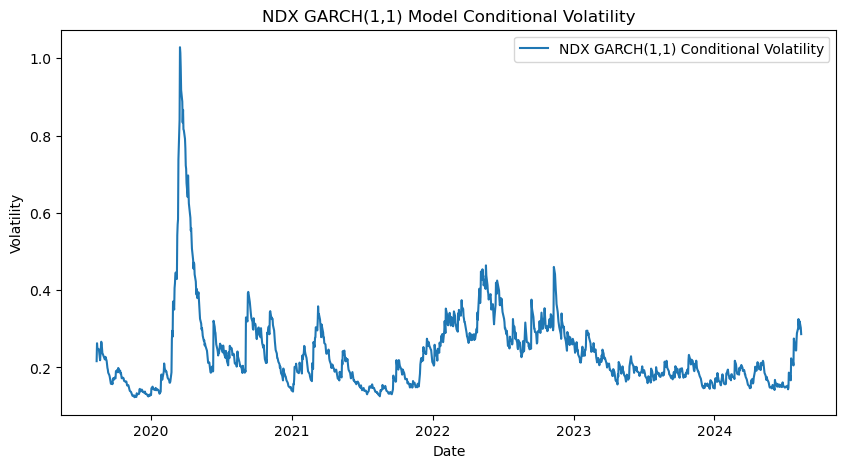
Figure 6: NDX Conditional Volatility Based on the GARCH(1,1) Model

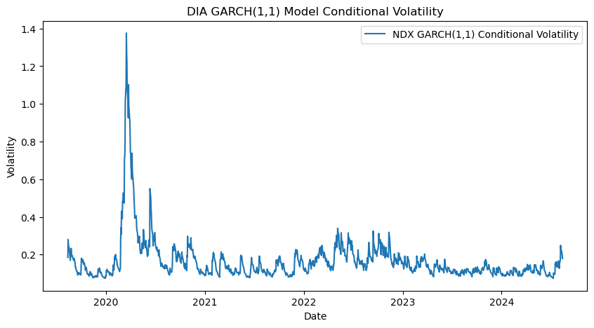
Figure 7: DIA Conditional Volatility Based on the GARCH(1,1) Model

Calculated the conditional volatility for the SPX, NDX, and DIA indices, this study applied the GARCH-fitted conditional volatility to the BS model for Monte Carlo simulations. Using the same data and options as the original BSM model, the option prices for the SPX, NDX, and DIA indices were obtained with the GARCH-fitted volatility. The pricing trends of the options for these three indices are illustrated in Figure 8, Figure 9, and Figure 10.

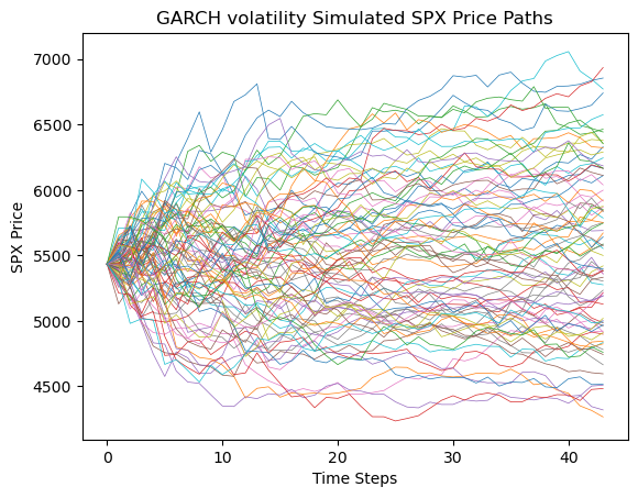
Figure 8: GARCH volatility simulated SPX price paths.

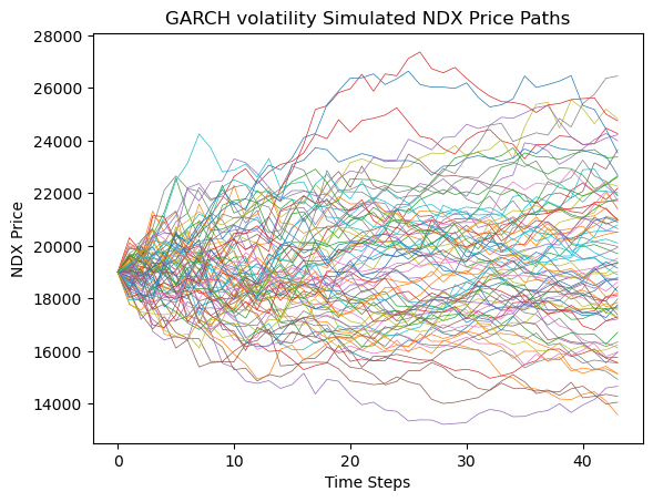
Figure 9: GARCH volatility simulated NDX price paths.

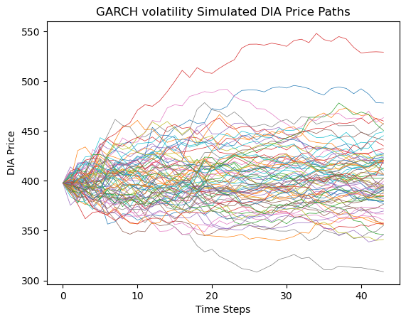
Figure 10: GARCH volatility simulated DIA price paths

Table 4, Table 5, and Table 6 presents the pricing forecasts for options on the three indices across various strike prices following the optimization of the GARCH model:

Table 4: SPX Option Pricing Across Varying Strike Prices

Table 5: NDX Option Pricing Across Varying Strike Prices

Table 6: DIA Option Pricing Across Varying Strike Prices

3.3. The RMSE Value Comparison

After computing the option prices for the SPX, NDX, and DIA index options, this study computed the RMSE (Root Mean Square Error) for the three indices based on data derived from the original BSM and the GARCH-optimized models. After calculating the option prices using two different methods, this study will retrieve the actual market prices of options with the same maturity date and similar transaction times from Yahoo Finance. The real market prices will then be compared with the option prices derived from the two models, and the RMSE will be calculated to assess the pricing accuracy of both methods. The results are presented below (Table 7):

Table 7: Comparison of RMSE of Two Methods

The study results indicate that for the SPX and DIA indices, the RMSE values were reduced by 7.27% and 16.83%, respectively, after applying the GARCH model optimization. This reduction in RMSE indicates that the GARCH model more accurately captures the dynamic volatility patterns present in these indices, leading to better alignment with the actual market prices of the options. In contrast, for the NDX index, the RMSE value after GARCH optimization did not decrease compared to the original BSM model, suggesting that the GARCH model did not significantly enhance pricing accuracy for the NDX index.

The result reflects the suitability of the GARCH model for indices dominated by industrial and consumer goods companies, where volatility is more stable and follows predictable patterns over time. In contrast, the NDX index results, primarily composed of technology companies, present a different picture. The RMSE value for NDX after applying the GARCH optimization did not show any significant reduction compared to the original BSM model. This suggests that the GARCH model does not provide a meaningful enhancement in capturing the volatility structure of the NDX index. Given that technology stocks are known for their high volatility and often exhibit sudden, nonlinear price movements, it is possible that the GARCH model, which is more suited for time-varying but smoother volatility, needs to effectively model the erratic and jumpy behavior of the tech sector options.

4. Discussion

This study empirically analyzed option pricing optimization for three major indices in the U.S. financial markets—SPX, NDX, and DIA—using both the BS and GARCH-optimized models. The final RMSE results indicate that the RMSE values for SPX and DIA based on GARCH optimization were significantly lower than those without GARCH optimization. However, the RMSE for NDX after GARCH optimization did not outperform the RMSE of the unoptimized NDX.

Upon analysis, this study attributes these findings to several vital factors. The DJIA and SPX are primarily composed of traditional industrial companies and financial firms—mature sectors with relatively low volatility. These sectors typically exhibit strong volatility clustering effects, a characteristic that GARCH models are particularly adept at capturing. Hence, GARCH models can effectively model the natural movement of volatility; they yield better-fitting results for these indices.

On the other hand, the NASDAQ-100 Index (NDX) is heavily comprised of leading technology companies like Apple, Microsoft, and Nvidia. These companies driven by innovation have to face intense market competition and technological revolution, resulting in volatility that is more significantly influenced by sudden events or breaking news. The volatility clustering effect is less evident in the technology sector than in traditional industries. Tech stocks often exhibit abrupt and irregular volatility, making it challenging for the GARCH model to effectively capture these complex and erratic volatility patterns.

Furthermore, the constituent companies of DJIA and SPX operate in relatively stable industry sectors, where macroeconomic factors, including interest rates, inflation, and GDP growth, influence volatility more. These macro variables tend to change gradually, resulting in smoother volatility dynamics that GARCH models are better adapted to predict by analyzing past fluctuations. On the other hand, most of the NASDAQ-100's constituent companies are high-growth, high-risk tech firms highly sensitive to market sentiment, technological breakthroughs, and geopolitical events. Their volatility can experience sudden spikes or declines, displaying jump behaviors and nonlinear characteristics, leading to less accurate fits.

In conclusion, GARCH models are effective for DIA and SPX primarily because the volatility of these indices reflects a more evident clustering effect and smoother dynamic characteristics attributed to the primary industries of the selected companies. However, the NASDAQ-100 index, due to the high volatility, jump behavior, and asymmetry of its tech stocks, presents challenges for the GARCH model in effectively capturing its volatility patterns.

5. Conclusion

This study conducted an empirical analysis of option pricing using both the BS and GARCH-enhanced models, focusing on major U.S. indices. The aim was to evaluate the effectiveness of integrating GARCH models into option pricing, mainly through Monte Carlo simulations for European call options using the GARCH model.

The results show that the incorporating method significantly improves option pricing accuracy for indices dominated by industrial and manufacturing companies, such as the DIA and SPX, which have more stable volatility patterns. However, the GARCH model did not significantly improve the NASDAQ-100, which consists mainly of high-growth tech companies with volatile and unpredictable behavior. The listed companies in NASDAQ-100 are more sensitive to market shocks, making it difficult for the GARCH model to predict such volatility.

To increase research efficiency and reduce the probability of errors in practice, this study only utilized the GARCH(1,1) model and did not explore more advanced models. This study reasonably assumes that adopting more complex and precise models like EGARCH and TGARCH models can further enhance the accuracy of option pricing and address the limitations observed in this study, particularly in the technology sector. Therefore, future research is recommended to use more advanced volatility models to enhance the accuracy of option pricing across different industries.

References

[1]. Black, F., & Scholes, M. (1973). The pricing of options and corporate liabilities. Journal of political economy, 81(3), 637-654.
[2]. Tong, T. (2023). Enhancing Option Pricing Accuracy through Empirical Performance: A GARCH-Based Approach to Refining Volatility Assumptions in the Black-Scholes Model. Highlights in Business, Economics and Management, 22, 75-82.
[3]. Bayraktar, E., & Poor, H. V. (2005). Arbitrage in fractal modulated Black–Scholes models when the volatility is stochastic. International Journal of Theoretical and Applied Finance, 8(03), 283-300
[4]. Lahouel, N., & Hellara, S. (2020). Improving the option pricing performance of GARCH models in inefficient market. Investment Management and Financial Innovations, 17(2), 14-25.
[5]. Bollerslev, T., Engle, R. F., & Nelson, D. B. (1994). ARCH models. Handbook of econometrics, 4, 2959-3038.
[6]. Duan, J. C. (1995). The GARCH option pricing model. Mathematical finance, 5(1), 13-32.
[7]. Bhat, A., & Arekar, K. (2016). Empirical performance of Black-Scholes and GARCH option pricing models during turbulent times: The Indian evidence. International Journal of Economics and Finance, 8(3), 123-136.
[8]. Barone-Adesi, G., Engle, R. F., & Mancini, L. (2008). A GARCH option pricing model with filtered historical simulation. The review of financial studies, 21(3), 1223-1258.
[9]. Thomas, P. (2001). A relationship between technology indicators and stock market performance. Scientometrics, 51, 319-333.
[10]. Rahman, S. (2001). The introduction of derivatives on the Dow Jones Industrial Average and their impact on the volatility of component stocks. Journal of Futures Markets: Futures, Options, and Other Derivative Products, 21(7), 633-653.
Cite this article
Zhao,H. (2024). Enhancing Option Pricing Accuracy: Integrating the GARCH Model into the Black-Scholes Model for U.S. Stock Indices. Advances in Economics, Management and Political Sciences,118,87-100.
Data availability
The datasets used and/or analyzed during the current study will be available from the authors upon reasonable request.
Disclaimer/Publisher's Note
The statements, opinions and data contained in all publications are solely those of the individual author(s) and contributor(s) and not of EWA Publishing and/or the editor(s). EWA Publishing and/or the editor(s) disclaim responsibility for any injury to people or property resulting from any ideas, methods, instructions or products referred to in the content.
About volume
Volume title: Proceedings of the 3rd International Conference on Financial Technology and Business Analysis
© 2024 by the author(s). Licensee EWA Publishing, Oxford, UK. This article is an open access article distributed under the terms and
conditions of the Creative Commons Attribution (CC BY) license. Authors who
publish this series agree to the following terms:
1. Authors retain copyright and grant the series right of first publication with the work simultaneously licensed under a Creative Commons
Attribution License that allows others to share the work with an acknowledgment of the work's authorship and initial publication in this
series.
2. Authors are able to enter into separate, additional contractual arrangements for the non-exclusive distribution of the series's published
version of the work (e.g., post it to an institutional repository or publish it in a book), with an acknowledgment of its initial
publication in this series.
3. Authors are permitted and encouraged to post their work online (e.g., in institutional repositories or on their website) prior to and
during the submission process, as it can lead to productive exchanges, as well as earlier and greater citation of published work (See
Open access policy for details).