1. Introduction

The NASDAQ Composite Index is a vital barometer market trends, encompassing a diverse array of companies primarily in the technology sector [1]. Forecasting the movements of the NASDAQ Composite Index is of paramount importance for investors, financial analysts, and policy-makers. Accurate predictions can guide investment strategies, risk management, and economic planning. However, forecasting the NASDAQ poses significant challenges due to the index's inherent volatility and the influence of numerous factors, including macroeconomic indicators, global events, and technological advancements. The dynamic and unpredictable nature of the stock market necessitates the use of robust analytical models to anticipate future trends effectively [2].

This study utilizes data sourced from Yahoo Finance, focusing on the monthly closing prices of the NASDAQ Composite Index from September 2019 to August 2024. The chosen timeframe encompasses a period of significant market activity, including the global influence of the COVID-19 and subsequent economic recovery. The dataset captures the overall upward trend in the index, alongside periods of volatility, reflecting the resilience and growth potential of the sectors represented. To accurately forecast the NASDAQ index, this study applies three distinct analytical models: Exponential Smoothing (ETS), Autoregressive Integrated Moving Average (ARIMA), and Linear Regression. Each model offers a unique approach to time series forecasting. By utilizing these various models, the study expects to provide a exhaustive evaluation of their predictive performance and to identify the most appropriate model for forecasting the NASDAQ index. The fundamental objective of this research is to evaluate the performance of these models in capturing the potential patterns of the NASDAQ Composite Index and to assess their forecasting accuracy. This evaluation is based on criteria such as the Root Mean Squared Error (RMSE) and Akaike Information Criterion (AIC), which provide quantitative measures of model performance. The results of this study have the potential to offer valuable guidance for investors and analysts in developing more informed and strategic approaches to market forecasting.

In this paper, Section 2 introduces the data sources and the specific characteristics of the NASDAQ Composite Index that are relevant for forecasting. Section 3 presents the methodology, detailing the three analytical models used—Exponential Smoothing, Autoregressive Integrated Moving Average, and Linear Regression. In Section 4, the results of each model are analyzed, with performance metrics such as Root Mean Squared Error and Akaike Information Criterion used for evaluation. Section 5 offers a comparative evaluation, highlighting the advantages and disadvantages of each model. Finally, Section 6 concludes with the implications of the findings and gives the suggestion about future for research aimed at enhancing the accuracy of financial forecasting models.

2. Dataset

The data was obtained from Yahoo Finance and relates to the NASDAQ Composite Index (IXIC). The NASDAQ is a market capitalization-weighted index, meaning its components are weighted according to their total market value, encompassing nearly all stocks listed on the Nasdaq exchange, one of the largest electronic stock exchanges globally [3]. The index covers over 2,500 companies across various sectors including technology, Consumer Discretionary, Healthcare, Industrials, etc. Given its heavy weighting in tech and growth stocks, the NASDAQ Composite can provide early signals about market trends and investor confidence in future economic growth, innovation, and technological advancements. This makes it an essential tool for investors looking to assess market sentiment and make well-informed investment decisions. The chosen data captures stock prices from September 2019 to August 2024, containing monthly closing prices.

By using the R programming, an overview of its performance over the given period are provided. The visualization of NASDAQ Composite Index closing price shown in the Figure 1.

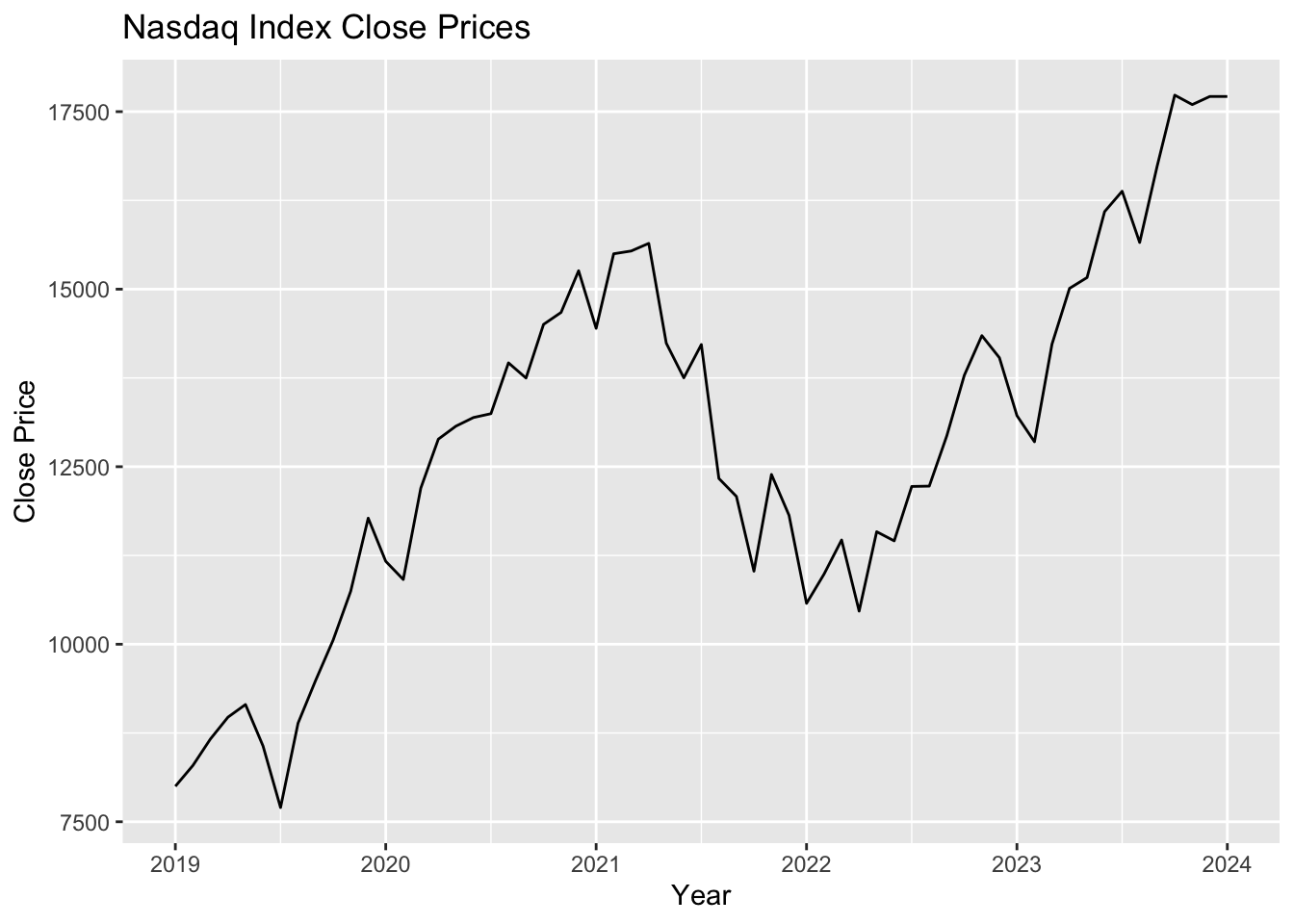
Figure 1: Time series plot of Nasdaq. (Picture Credit: Original)

There is a clear overall trend of going up in the NASDAQ over the observed period. The index starts below 10,000 in 2019 and reaches above 17,500 by 2024. The index shows periods of volatility, with several notable peaks and troughs, demonstrating resilience and investor confidence in the technology and growth sectors.

Then applying the Residual test to check whether the chosen Nasdaq Index is white noise or not.

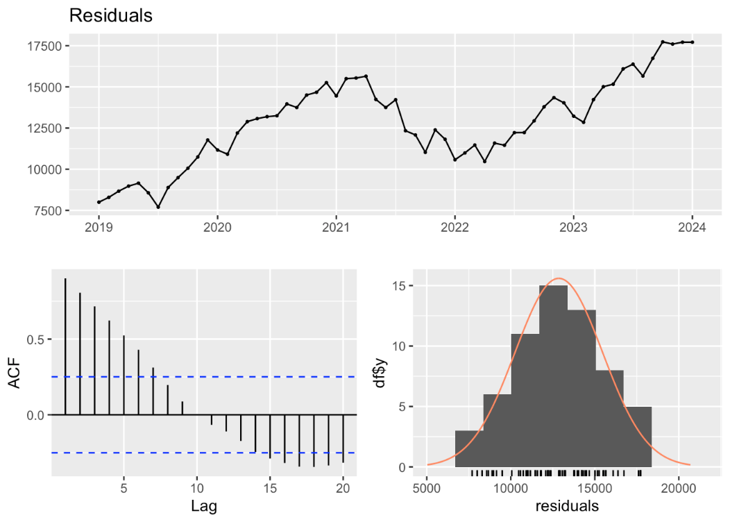
Figure 2: Residual test of NASDAQ (Picture Credit: Original)

The residual plot (top left) in Figure 2 shows that while the residuals changes around zero, indicating the model captures the general trend of the NASDAQ Composite Index, there is still some autocorrelation and a trend present. The ACF plot (bottom left) reveals significant autocorrelations at several lags, especially in the initial lags, indicating that the residuals do not exhibit white noise behavior. This indicates that the model has not fully caught all potential patterns in the data, highlighting the need for further adjustments or the use of a more advanced model to address these autocorrelations. To be more precise about the above consideration, the Ljung-Box test is necessary to be applied.

Table 1: Ljung-Box test of Residuals.

The Ljung-Box test results show a Q* value of 197.79 with a p-value of less than 2.2e-16, which is significant. This indicates that there exists a notable autocorrelation present in the residuals, confirming that the residuals of the model are not purely random and white noise.

Therefore, to remove any autocorrelation, applying differencing to stabilize the mean and variance over time.

Begin

log_ts_data <- log(ts_data)

diff_ts_data <- diff(log_ts_data)

End.

Now, rechecking the residuals which shown in Figure 3.

Figure 3: Residual test of differenced NASDAQ. (Picture Credit: Original)

After differencing, the model appears to have addressed the initial autocorrelation and trend issues in the residuals. Then, the Ljung-Box test shows that:

Table 2: Ljung-Box test of differenced Residuals.

The Ljung-Box test statistic Q∗=8.3267Q with 12 df and a p-value of 0.7591 indicates that the residuals are not significantly different from white noise. A high p-value, which is greater than 0.05, means that there is no significant autocorrelation remaining in the residuals. This result, combined with the visual analysis of the ACF plot, confirms that differencing the data has effectively removed autocorrelation, implying that the model is now more appropriately specified for the data.

3. Model

3.1. Rationale for Model Selection

This study selects three models for predicting the NASDAQ index: ETS, Linear Regression, and ARIMA. These models were chosen due to their distinct approaches to time series forecasting and their ability to capture different characteristics of the data. By using these diverse models, a comprehensively evaluation of their predictive performance on the NASDAQ index will be offered.

3.2. Exponential Smoothing (ETS)

The Exponential Smoothing model is a versatile method for time series forecasting, especially well-suited for handling data that exhibits patterns involving trends and seasonality. It combines three components—Error (E), Trend (T), and Seasonality (S)—in various ways to suit different data characteristics [4]. In this study, the ETS model was used to differenced NASDAQ time series data to handle non-stationarity by removing trends. The model fitting was done using the ets() function in R, which selects the most optimal model based on the data. The model’s summary statistics were then reviewed to evaluate its components and forecasting accuracy.

3.3. Autoregressive Integrated Moving Average (ARIMA)

The Autoregressive Integrated Moving Average model is a commonly applied technique for time series forecasting, particularly effective for handling non-stationary data. ARIMA is characterized by three key parameters: autoregressive order, differencing degree, and moving average order. Differencing (d) represents an important role in making the time series stationary, an essential step for effective ARIMA modeling [5]. In this study, the ARIMA model was applied to differenced NASDAQ time series data to address non-stationarity. The differencing process removes trends and seasonality, stabilizing the mean. The auto.arima() function in R was used to automatically select the optimal ARIMA model by tuning p, d, e based on criteria like AIC.

3.4. Linear Regression

Linear regression is a fundamental statistical technique used to model the relationship between a dependent variable and more independent variables [6]. In this study, a simple linear regression model was used to the differenced NASDAQ index data to identify linear trends over time. Differencing the data removed non-stationarity, allowing the model to focus on the underlying linear patterns. A time index variable was created to represent the sequence of the differenced data points. The model was fitted using the lm() function in R, with the differenced NASDAQ data as the response variable and the time index as the independent variable, capturing any linear trends present in the data.

3.5. Model Validation

The data was separated into training and testing sets to evaluate the predictive performance of each model. The training set was used to fit the models and tune their parameters, while the testing set served as a benchmark to assess out-of-sample prediction accuracy. Cross-validation techniques were applied to ensure strong model evaluation. Performance Metrix Root Mean Squared Error is used to compare the models' predictive capabilities and generalizability to unseen data, which is calculated by:

\( RMSE= \sqrt[]{\sum _{i=1}^{n}\frac{ {(\hat{{y_{i}}}-{y_{i}})^{2}}}{n}} \) (1)

Where \( \hat{{y_{1}}},\hat{{y_{2}}},\hat{{y_{3}},}…\hat{{y_{n}}} \) are predicted value, \( {y_{1}}{,{y_{2}},y_{3}},…,{y_{n}} \) are observed values, n is the number of observed values.

4. Results Analysisw

4.1. ETS Model Results

The ETS model, ETS (A,N,N), was fitted to the differenced NASDAQ data. This model configuration suggests that the data was best represented with an additive error, no trend, and no seasonality, which should use Simple Exponential Smoothing formula for forecasting shown in Figure 4:

\( {\hat{y}_{t+1}}=α{y_{t}}+(1-α)​{\hat{y}_{t}} \) (2)

In this equation, \( {\hat{y}_{t+1}} \) represents the forecast for the next time, \( α \) is the smoothing parameter, \( {y_{t}} \) means the actual value at time t, and \( {\hat{y}_{t}} \) means the forecasted value at time t.

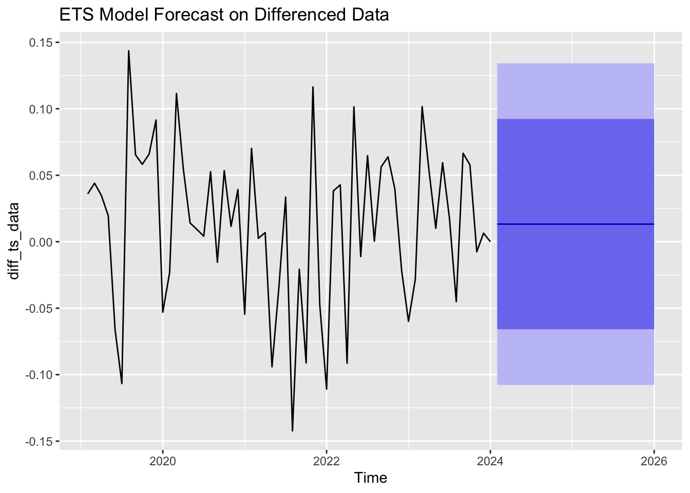
Figure 4: ETS 24-month forecasting plot. (Picture Credit: Original)

4.2. ARIMA Model Results

The ARIMA model was ARIMA (0,0,0) with a non-zero mean, effectively modeling the differenced data as a stationary process with constant mean. The formula used to forecast ARIMA is:

\( ϕ(B){(1-B)^{d}}{y_{t}}=θ(B){ϵ_{t}} \) (3)

Where \( ϕ(B) \) is the AR terms, \( {(1-B)^{d}} \) represents differencing d times, \( θ(B) \) is the MA terms, B is the backshift operator, and \( {ϵ_{t}} \) is white noise as Figure 5 shown below.

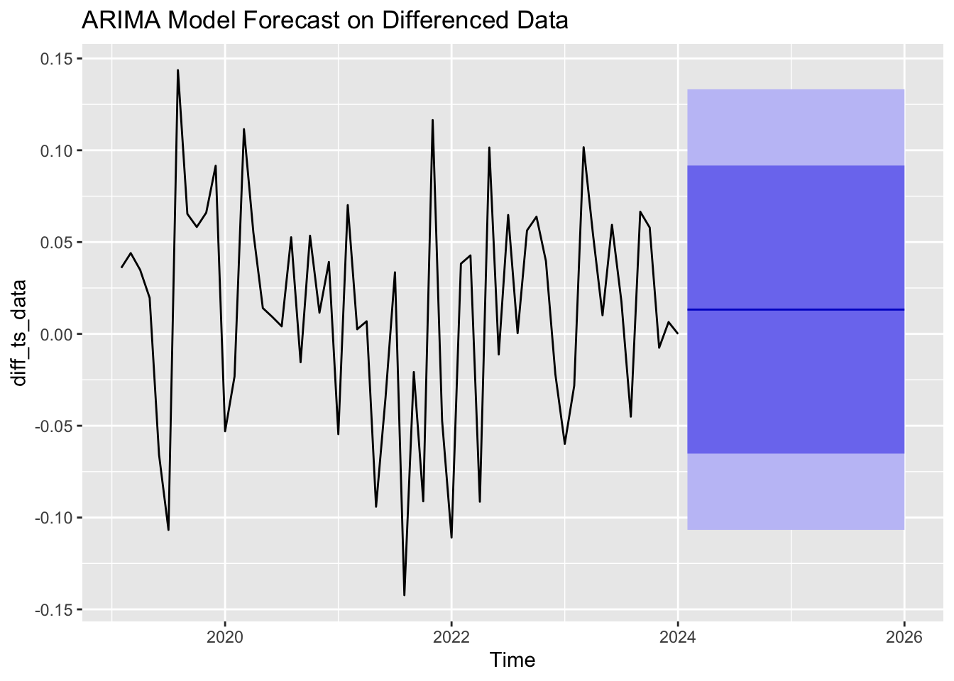
Figure 5: ARIMA 24-month forecasting plot. (Picture Credit: Original)

4.3. Linear Regression Model Results

The linear regression model was applied to the differenced NASDAQ data to identify any residual linear trends. With the formula:

\( {y_{t}}={β_{0}}+{β_{1}}{x_{t}}+{ϵ_{t}} \) (4)

Where \( {β_{0}} \) represents the intercept, \( {β_{1}} \) means the slope, \( {x_{t}} \) is independent variable, \( {ϵ_{t}} \) is the error term.

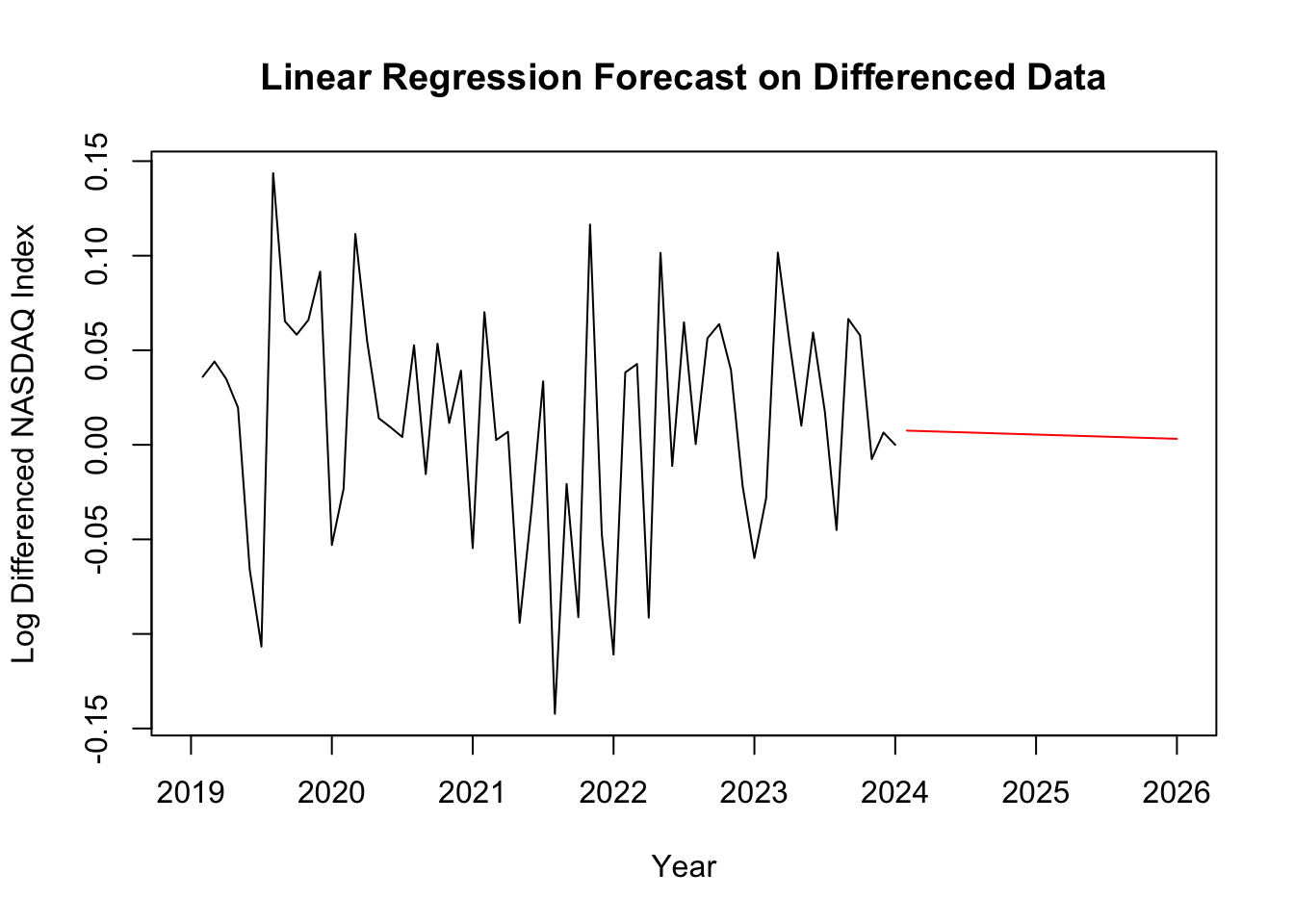
Figure 6: Linear Regression forecasting plot. (Picture Credit: Original)

The linear regression forecast model in Figure 6 appears as a flat or slightly declining red line. This suggests that the model predicts that the future values of the log-differenced NASDAQ Index will not change significantly, remaining relatively constant or slightly decreasing over time.

4.4. Comparative Results

To assess the forecasting performance for the three models—ETS, ARIMA, and Linear Regression—each was trained on 80% of the differenced NASDAQ index data, with the remaining 20% used for testing. The models were examined using the Root Mean Squared Error on the test data to measure their predictive accuracy.

Table 3: RMSE Value of three models.

From Table 3, the RMSE values indicate that both the ETS and ARIMA models outperformed the Linear Regression model in terms of forecast accuracy on the test data, effectively managing the differenced NASDAQ data's trends and variability. In contrast, the Linear Regression model, while useful for understanding linear trends, did not perform as well due to its simpler structure and lack of ability to capture the nuances in the data.

Since it could be difficult to determine which model provides the best forecasting ability based on the RMSE values are shown above, the study then checks the AIC value for those two models shown in Table 4.

Table 4: AIC Value.

By comparing, ARIMA model fits the Nasdaq Index better with the lower AIC value.

The AIC and RMSE results together provide a comprehensive view of model performance. The ARIMA model [7-8], which has the lowest AIC and competitive RMSE, was the best overall model, balancing model fit and forecast accuracy. The ETS model, having the slightly higher AIC, also provided accurate forecasts with a low RMSE [9-10]. The Linear Regression model, although simple and having a similar AIC to the ARIMA model, was less effective in terms of forecast accuracy, indicating that it does not adequately capture the sophisticaty of financial time series data like the NASDAQ index.

5. Conclusion

This study set out to forecast the NASDAQ Composite Index using three distinct analytical models: Exponential Smoothing, Autoregressive Integrated Moving Average, and Linear Regression. The motivation behind this research was to determine which model offers the most reliable forecasting capability for the NASDAQ index, an essential benchmark for gauging market trends, particularly in the technology and growth sectors. The analysis was conducted on monthly closing prices from September 2019 to August 2024, a period marked by significant market fluctuations and events like the global COVID-19.

The ETS model, with its ability to accommodate trends and seasonality, provided a relatively accurate forecast, showing that the index could be well-represented with an additive error, no trend, and no seasonality. The ARIMA model, however, emerged as the most effective in capturing the complexities of the NASDAQ index, as indicated by its lower Akaike Information Criterion value and competitive Root Mean Squared Error. This suggests that ARIMA's approach to modeling non-stationary data with its differencing technique is particularly suited to financial time series data, which often exhibit volatility and autocorrelation.

In contrast, the Linear Regression model, while useful for understanding simple linear trends, did not perform as well in this context. Its higher RMSE indicated that it could not capture the more intricate patterns and volatility present in the NASDAQ data. This result underscores the limitations of using a purely linear approach for forecasting a complex financial index, where nonlinear trends and autoregressive components play a significant role.

The comparative analysis of these models emphasizes the significance of choosing a suitable forecasting approach that aligns with the properties of the data. The superior performance of the ARIMA model demonstrates its robustness in handling non-stationary time series and its ability to provide more accurate forecasts in the context of the NASDAQ index. This finding has practical implications for investors, analysts, and policymakers, suggesting that employing more sophisticated models like ARIMA can lead to better-informed decision-making and risk management.

However, this study is not without limitations. While ARIMA and ETS provided reasonably accurate forecasts, there is always an element of uncertainty in financial markets due to unforeseen events and market dynamics. The chosen models are based on data from the past and their predictive power may vary with changing market conditions. Then, the current dataset includes only daily closing prices. It might be worth exploring how RC performs with different data intervals, such as hourly, or even high frequencies time scales. Future studies could investigate more sophisticated models, including machine learning-based techniques or ensemble methods, to further improve forecasting precision. Moreover, integrating external elements like macroeconomic indicators, interest rates, and global political events may offer a more comprehensive perspective and potentially boost model performance.

In conclusion, the study offers important insights into the predictive strengths of diverse time series models for the NASDAQ Composite Index. By recognizing ARIMA as the most effective model in this case, it establishes a basis for more precise market forecasting and informed investment strategies. The results highlight the importance of choosing models that are well-suited to the specific traits of financial data and open the door to future research on more advanced forecasting techniques.

References

[1]. Frankel Matthew. What is the Nasdaq Composite Index? The Motley Fool, 2024.
[2]. Arashi Mohammad, and Rounaghi Mohammad Mahdi. Analysis of market efficiency and fractal feature of NASDAQ stock exchange: Time series modeling and forecasting of stock index using ARMA-GARCH model. Springer Open, 2022.
[3]. Chen Ames. What Does the Nasdaq Composite Index Measure? Investopedia, 2023.
[4]. Franco Daniel. Exponential Smoothing Methods for Time Series Forecasting. Encore, 2022.
[5]. Hayes Adam. Autoregressive Integrated Moving Average (ARIMA) Prediction Model. Investopedia, 2024.
[6]. Needle Flori. How to Use Regression Analysis to Forecast Sales: A Step-by-Step Guide. HubSpot, 2021.
[7]. Ristanoski Goce, Liu Wei, Bailey James. Time Series Forecasting Using Distribution Enhanced Linear Regression. Pp. 484-495. 2013.
[8]. Contreras J, Espinola R, Nogales F.J, Conejo A.J. ARIMA Models to Predict Next-day Electricity Prices. 2003.
[9]. Wang Weijia, Tang Yong, Xiong Jason, and Zhang Yicheng. Stock market index prediction based on reservoir computing models. ScienceDirect, 2021.
[10]. Huang Jingxuan and Hung Juichung. Forecasting Stock Market Indicies using PVC – SVR. Springer Link, 89-96, 2014.
Cite this article
Cao,L. (2024). Forecasting the NASDAQ Index - Based on Diversified Analytical Models. Advances in Economics, Management and Political Sciences,140,30-39.
Data availability
The datasets used and/or analyzed during the current study will be available from the authors upon reasonable request.
Disclaimer/Publisher's Note
The statements, opinions and data contained in all publications are solely those of the individual author(s) and contributor(s) and not of EWA Publishing and/or the editor(s). EWA Publishing and/or the editor(s) disclaim responsibility for any injury to people or property resulting from any ideas, methods, instructions or products referred to in the content.
About volume
Volume title: Proceedings of ICFTBA 2024 Workshop: Finance's Role in the Just Transition
© 2024 by the author(s). Licensee EWA Publishing, Oxford, UK. This article is an open access article distributed under the terms and
conditions of the Creative Commons Attribution (CC BY) license. Authors who
publish this series agree to the following terms:
1. Authors retain copyright and grant the series right of first publication with the work simultaneously licensed under a Creative Commons
Attribution License that allows others to share the work with an acknowledgment of the work's authorship and initial publication in this
series.
2. Authors are able to enter into separate, additional contractual arrangements for the non-exclusive distribution of the series's published
version of the work (e.g., post it to an institutional repository or publish it in a book), with an acknowledgment of its initial
publication in this series.
3. Authors are permitted and encouraged to post their work online (e.g., in institutional repositories or on their website) prior to and
during the submission process, as it can lead to productive exchanges, as well as earlier and greater citation of published work (See
Open access policy for details).