1. Introduction

With the deepening of global economic integration, the stock market has become a key indicator to reflect the macroeconomic dynamics. There is an increasing demand for stock market forecasting from investors and policymakers, especially in the context of increasingly interconnected global markets.

Time series models are widely used in stock market prediction, especially ARIMA model and ETS model, which are excellent in capturing market fluctuations and trends. Different models are suitable for different market environments [1-2]. Hansen's research shows that ARIMA model shows high prediction accuracy when processing financial data with long-term trends, especially for time series with strong autocorrelation [3]. The ETS model, by combining trends, seasonality and error terms, is suitable for short-term forecasting, especially in financial markets [4]. Hyndman et al. pointed out that ETS model has unique advantages in capturing non-linear market fluctuations and can cope with complex market dynamics [5]. By comparing the performance of ARIMA and ETS models in China's stock market, Fan and Yin found that there are differences in the prediction accuracy of the two models under different market conditions, indicating that selecting the right model is crucial to the accuracy of prediction [6]. In order to further explore the correlation and future trend of Chinese and American stock markets, this paper adopts ARIMA model and ETS model to analyze and forecast Shanghai Composite Index and Nasdaq Index respectively. The ARIMA model first proposed by Box and Jenkins has been widely used in financial markets, and recent studies also show that, The ETS model performs well under certain conditions [7]. By comparing the predicted results of the two models, this paper aims to reveal the likely future volatility trends of the Chinese and American stock markets and provide decision support for investors. By comparing the prediction accuracy of the two models, the applicability of different models in Chinese and American stock markets is discussed. At the same time, this paper will also analyze the future volatility trends of these two markets in the context of the global economy to provide more forward-looking references for investors.

2. Data

This study uses the monthly price data of Nasdaq Composite Index and Shanghai Composite Index. The data, sourced from the website investing, covers a time frame of 122 months of observations from January 2014 to December 2023.

In the process of data processing, the date format is first converted and only the year part is reserved for the construction of the time series. To facilitate the modeling analysis, the data is adjusted from daily prices to monthly prices. The processed data contains 12 observations per year at a monthly frequency. When the missing values were checked, no missing values were found, so no further data cleaning was required.

Next, the data is divided into a training set and a test set. The first 90 months of data (January 2014 to December 2021) were used to train the model, and the second 32 months of data (January 2022 to December 2023) were used for model prediction and evaluation.

For the Shanghai Composite Index, the lowest price is 2026, the highest is 4612, the average is 3103, and the median is 3136. The data show that the price of the Shanghai Composite Index is generally concentrated around 3000 points, the fluctuation range is relatively moderate, the difference between the highest and the lowest value is relatively small, indicating a relatively stable market performance.

The Nasdaq index showed more volatility, with a low of 4,104, a high of 15,645, an average of 8,604 and a median of 7,602. This shows that the price volatility of the Nasdaq index during the observation period is significantly higher than that of the Shanghai Composite Index, especially in the higher price range, reflecting greater market volatility and possibly higher risks (See Table 1).

Table 1: Data description Statistics

3. Method

3.1. ARIMA model

The autoregressive integral moving average (ARIMA) model is a widely used statistical method for time series data. By taking into account historical trends, seasonality, and noise in the data, it is able to effectively capture patterns in time series and make short-term predictions. ARIMA models are good at dealing with time series with non-stationarity. By differentiating the data, the model can be transformed into a stationary form, so as to apply linear regression and other methods to make predictions. The ARIMA model consists of three main parts: autoregressive (AR) term, difference (I) term, and moving average (MA) term. Its general form is ARIMA (p, d, q): The ARIMA model consists of three main parts: autoregressive (AR) term, difference (I) term, and moving average (MA) term. Its common form is ARIMA (p, d, q) (See Equation (1)) [8-10].

In this case \( {Y_{T}} \) is the value of the time series; \( {φ_{1}},{φ_{2}},…,{φ_{p}} \) is the autoregressive coefficient; \( {θ_{1}},{θ_{2}},…,{θ_{q}} \) is the moving average coefficient; \( {ε_{t}} \) is white noise; \( d \) is the difference number, representing the difference process that turns a time series into a stationary one.

The process of ARIMA model construction is as follows: 1. Model identification and selection: Firstly, by drawing autocorrelation function (ACF) and partial autocorrelation function (PACF) graphs, the order of AR and MA terms are preliminarily determined, namely parameters ppp and qqq. The difference degree ddd is determined by a unit root test such as an ADF test. 2. Parameter estimation: Estimate parameters by maximum likelihood estimation (MLE) or least square method. 3. Model test: test the independence and normality of the model residuals to ensure that the residuals have no autocorrelation. 4. Prediction: Make predictions about future data based on fitted models.

3.2. ETS model

The ETS model (error, Trend, seasonality model) is a time series forecasting model based on an exponential smoothing method. By capturing the trend, seasonality and error terms of data, this method is suitable for modeling and forecasting stationary and non-stationary time series. The strength of the ETS model is its ability to handle seasonal changes, suitable for financial market data with periodic fluctuations The ETS model generates different model structures based on different combinations of these three, such as ETS (A, A, A) representing addition error, addition trend, and addition seasonality. The ETS model consists of three main components \( {Y_{t}}={T_{t}}+{S_{t}}+{E_{t}} \) . \( {T_{t}} \) represents the trend item in the time series; \( {S_{t}} \) represents a seasonal item; \( {E_{t}} \) represents the error term. The ETS model generates different model structures based on different combinations of these three items, such as ETS (A, A, A) representing addition error, addition trend, and addition seasonality. The ETS model construction process is as follows: First, model selection, through the automated ETS algorithm, selects the most suitable model combination of data characteristics (trend, seasonality). Parameter estimation: Estimate model parameters using least squares or exponential smoothing based on the trend and seasonality of the data. Model testing: The residual is tested to ensure good model fitting. Prediction: The ETS model is used to make predictions about future data points, taking into account seasonality and trend effects.

4. Result

4.1. Prediction Results

The chart below shows the forecast results for the Nasdaq and Shanghai indices. The red line represents the price index predicted by the model, and the black line is the actual price index. In Figure 1, the ARIMA model is used to make time series predictions for the Nasdaq index. The black line represents the actual historical data from 2014 to 2023, while the red line represents the model's prediction for the last year (2023). The blue area represents a 95% confidence interval, and a narrower confidence interval indicates that the model has a high degree of confidence in the short-term future. As can be seen in the chart, the ARIMA model captures the Nasdaq's downward trend well, but the forecast value is slightly lower than the actual observed data. As can be seen from the expansion of the shadow in Figure 2, the uncertainty of the forecast gradually increases over time. The extended range of the blue shading indicates that the confidence interval of the predicted value becomes wider and wider over time. This is a common feature of ETS models, showing that future market volatility and unforeseen factors make the forecast outcome uncertain as the forecast period extends. As for the market performance forecast, although historical data indicate a significant decline in the Nasdaq index, the ETS model's forecast indicates that future prices are likely to stabilize in 2022-2024 and will not continue to decline sharply as they have in the past few years. However, due to the wide confidence interval, there may still be large volatility in the market in the future. In summary, the ETS model exhibits a high degree of uncertainty in predicting future price trends, but based on current trends, it expects the NASDAQ index to remain at its current level in the future, and may even decline slightly, but not too drastically.

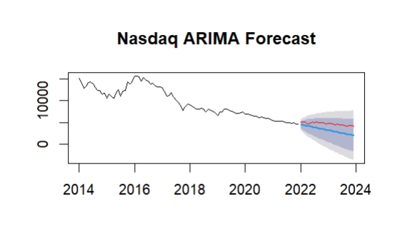
Figure 1: ARIMA model predictions for the Nasdaq index

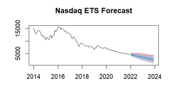
Figure 2: ETS model predictions for the Nasdaq Index

In Figure 3, the results of using the ARIMA model to forecast the Shanghai Composite Index. First from the trend analysis, from 2022 onwards, the red forecast line shows a significant downward trend. Model forecasts show that the index may continue to decline in the coming period, and the volatility is wide. At the same time, the grey shaded part of the figure represents the confidence interval, which gradually expands over time, showing the increased uncertainty of the model in predicting the forward value. This means that the models' predictions for the future may be far off. The chart shows that the forecast based on the ARIMA model indicates that the Shanghai Composite Index may have a relatively large decline in the future. In Figure 4, the ETS model's predictions are similar to those of the ARIMA model, which also shows a downward trend in the future. However, compared to the ARIMA model, the ETS model predicts a more gradual decline, with the index declining to level off after 2022. The confidence interval is also wide compared to the ARIMA model, which means that the ETS model is also uncertain about future predictions. Over time, the ETS model has a slightly wider confidence interval than the ARIMA model, indicating slightly less confidence in future trends. In practical application, the prediction results of ETS model show that the Shanghai Composite Index may show a downward trend in the future, but the decline speed and amplitude may be moderate. Because of the wide confidence interval, investors need to consider the uncertainty of the model and make decisions in conjunction with other information. The model is also suitable for short-term decisions, but the instability of long-term forecasts should be ignored.

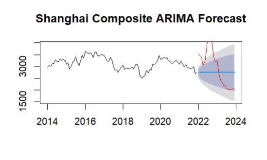
Figure 3: ARIMA model forecast results of Shanghai Composite Index

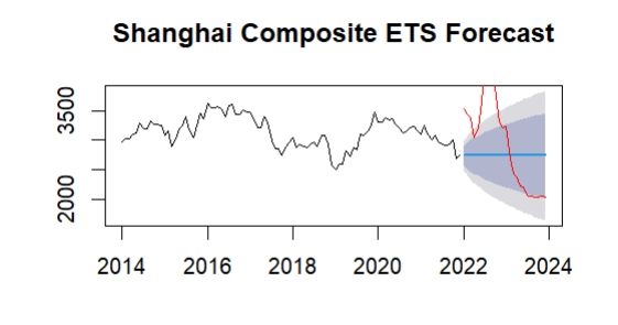
Figure 4: Shanghai Composite Index and ETS model predictions

4.2. Prediction Accuracy

Table 2 shows the mean square error of the ARIMA and ETS models in predicting the Nasdaq and Shanghai indices

Table 2: Precision results of RMSE and MSE

In Table 2, from the results of mean square error, it can be seen that the ARIMA model slightly outperforms the ETS model on the Nasdaq index, while the ETS model performs better on the Shanghai Index. This shows that Nasdaq index is more suitable for trend analysis, while SSE index is more seasonally influenced, so ETS model is more advantageous in predicting SSE index.

5. Conclusion

With increased volatility in global financial markets, accurate forecasting of asset prices is important for investors and policymakers. Given that the US is currently in a rate reduction cycle, it is particularly important to develop and evaluate accurate asset price forecasting models. In this paper, ARIMA model and ETS model are used to predict the time series of NASDAQ index and Shanghai Composite Index respectively. By comparing the prediction performance indexes of the two models, such as mean square error (MSE) and root mean square error (RMSE), it is found that ARIMA model has higher prediction accuracy in most cases. The results show that the performance of different models in different markets is different, which provides a basis for investors to choose the right forecasting model. This study provides valuable empirical analysis for the field of asset price forecasting, especially in the context of global economic uncertainty, and has important practical application value.

Future research could further explore the applicability of asset price forecasting models in other economies, particularly over different economic cycles. In addition, combining macroeconomic variables or using machine learning models for multi-model fusion forecasts may further improve the accuracy of forecasts. This will provide more powerful tools and support for asset management and risk control.

References

[1]. Liu, Z., & Li, H. (2020). Stock price forecasting based on ARIMA and GARCH models. Journal of Finance, 45(4), 563-575.
[2]. Box, G. E. P., & Jenkins, G. M. (1970). Time series analysis: Forecasting and control. Holden-Day.
[3]. Hansen, P. R. (2005). A comparison of the accuracy of ARIMA and ETS models in forecasting stock market returns. Journal of Financial Economics, 80(2), 396-405.
[4]. Taylor, J. W. (2003). Short-term electricity demand forecasting using double seasonal exponential smoothing. Journal of Operational Research Society, 54(8), 799-805.
[5]. Hyndman, R. J., & Khandakar, Y. (2008). Automatic time series forecasting: The forecast package for R. Journal of Statistical Software, 27(3), 1-22.
[6]. Fan, X., & Yin, W. (2019). Time series forecasting for stock market volatility: A comparison between ARIMA and ETS models. Finance Research Letters, 31, 122-128.
[7]. Box, G. E. P., & Jenkins, G. M. (1970). Time series analysis: Forecasting and control. Holden-Day.
[8]. Zhang, Y., & Wang, S. (2021). An empirical analysis of the impact of monetary policy on stock prices in China and the United States. Economic Research Journal, 58(3), 102-117.
[9]. Poon, S.-H., & Granger, C. (2003). Forecasting volatility in financial markets: A review. Journal of Economic Literature, 41(2), 478-539.
[10]. Chen, X., & Liu, L. (2020). The effects of interest rate changes on asset prices in the context of global financial markets. Journal of International Financial Markets, 28(1), 45-60.
Cite this article
Yuan,S. (2024). Nasdaq and Shanghai Composite Index Forecast Based on ARIMA and ETS Models. Advances in Economics, Management and Political Sciences,141,100-105.
Data availability
The datasets used and/or analyzed during the current study will be available from the authors upon reasonable request.
Disclaimer/Publisher's Note
The statements, opinions and data contained in all publications are solely those of the individual author(s) and contributor(s) and not of EWA Publishing and/or the editor(s). EWA Publishing and/or the editor(s) disclaim responsibility for any injury to people or property resulting from any ideas, methods, instructions or products referred to in the content.
About volume
Volume title: Proceedings of ICFTBA 2024 Workshop: Finance's Role in the Just Transition
© 2024 by the author(s). Licensee EWA Publishing, Oxford, UK. This article is an open access article distributed under the terms and
conditions of the Creative Commons Attribution (CC BY) license. Authors who
publish this series agree to the following terms:
1. Authors retain copyright and grant the series right of first publication with the work simultaneously licensed under a Creative Commons
Attribution License that allows others to share the work with an acknowledgment of the work's authorship and initial publication in this
series.
2. Authors are able to enter into separate, additional contractual arrangements for the non-exclusive distribution of the series's published
version of the work (e.g., post it to an institutional repository or publish it in a book), with an acknowledgment of its initial
publication in this series.
3. Authors are permitted and encouraged to post their work online (e.g., in institutional repositories or on their website) prior to and
during the submission process, as it can lead to productive exchanges, as well as earlier and greater citation of published work (See
Open access policy for details).