1.Introduction

In the formulation of sound economic policies and risk management, as well as investment decisions, risk analysis, and the precise prediction of asset prices are critical factors for investors, speculators, and policymakers. The information regarding the future prices of equities, bonds, and other commodities will also be beneficial to all stakeholders in the organization, as the prevailing market conditions are quite volatile. This is further exacerbated by volatility effects that are influenced by macroeconomic factors, geopolitical events, the company's performance, and investors' sentiment regarding asset returns [1]. In this type of environment, it is possible to analyze and verify that time series models are also effective for forecasting future asset prices by utilizing historical data. Financial time series analysis employs three varieties of models: Autoregressive (AR), Moving Average (MA), and Autoregressive Moving Average (ARMA).

AMF uses the observed values of data presented in a time series through the AR model to predict future observations. In contrast, it assumes that asset prices have fluctuated according to their historical value, regardless of the present or future. On the other hand, the MA model relies on its ability to use the misfit or error values from previous predictions to create new ones. The combination of these two functions renders ARMA a significantly more valuable forecasting instrument than either the autoregressive or moving average when utilized independently. A variety of financial sectors, including equities, commodities, bonds, and volatile crypto currencies, extensively employ these time series models [2]. Based on historical data and forecasting errors, these models are significantly more precise than any other model. The financial market has extensively implemented autoregressive time series-based forecasting models. Specifically discussed the AR, MA, and the modified model, ARMA.

Autoregressive (AR), Moving Average (MA), and Autoregressive Integrated Moving Average (ARIMA) are the most frequently employed time series models, as previously discussed in the literature. All markets have implemented basic models to generate financial time series forecasts. The equities, bonds, and commodities markets have been analyzed using AR, MA, and ARMA categories [3]. However, there is a lack of extensive research on the potential implementation of the aforementioned models in established markets like the United Kingdom or the United States.

The purpose of this paper is to demonstrate the pertinent application of AR, MA, and ARMA models in the forecasting of financial series data, with a particular emphasis on their efficiency and effectiveness. Underscores the significance of these models in the enhancement of forecasting accuracy and the conduct of market analyses. The study underscores the necessity of conducting a more thorough examination of these models, their efficacy in developed markets, and their susceptibility to market fluctuations [4].

2.Data and Methods

2.1.Data Source

In order to obtain an accurate trend of stocks from historical aspect, yahoo finance is used [5]. This study used statistical data from Yahoo Finance, a trusted and popular website. Yahoo Finance provides historical data on stocks, indices, commodities, and crypto currencies. Daily closing prices, opening prices, range, trading volume, and more for numerous assets are included. In addition to Yahoo Finance, the Federal Reserve Economic Data (FED) and World Bank provide interest rates and inflation estimates to ensure that the models incorporate the proper macro variables that may affect asset values.

2.2.Time Range

This research spans January 2010–December 2023. This 13-year research period was chosen for the following reasons. First, it can analyse bullish, bearish, and volatile phase situations. This expanded time frame allows the study to examine important market dynamics like the post-2008 financial crisis rebound, the volatility as markets tumbled in the 2011 European debt crisis, the long bull run in the 2010s, the rapid and severe declines caused by the 2020 COVID-19 pandemic, and the recovery to that point. The selected time span encompasses low and high market torque, making the dataset better for comparing AR, MA, and ARMA model accuracy in varied situations.

2.3.Selection Criteria

This study then identifies global market indices, including the S&P 500 index, which represents US markets. There are technology markets in the United States, the United Kingdom, and the United States. Given that it is unfeasible to optimize the efficacy of trading strategies for a specific set of parameters, it is logical to allow for a variety of analyses that are contingent upon market conditions. The indices selected based on their liquidity, capitalization, and geographical location [6].

3.Methodology

This section includes three primary time series models: autoregressive (AR), moving average (MA), and autoregressive moving average (ARMA) types.

3.1.AR Regression Model

The AR model analyzes past values derived from a time series. The financial industry. The previous stock's price determines future stock prices, and stock returns also exhibit autocorrelation. The AR model is appropriate for this purpose because there is a linear relationship between an asset's present value and the prior value scenario. The AR model is effective for financial forecasting when it focuses on short-term price movements in stable markets [7].

3.2.Moving Average (MA) Model

The Moving Average (MA) Model uses the link between future values and past mistakes (or shocks) to forecast, making it a powerful tool. Because prior forecast mistakes can explain variance, the MA model works well with random shocks or short-term volatility [8].

3.3.Autoregressive Moving Average (ARMA) Model

The ARMA model, as its name implies, combines the advantageous features of both the AR and MA models. It does so by modeling the past values and errors simultaneously, thereby enabling a more thorough understanding of the time series. The ARMA model is well-suited to financial markets that exhibit both autoregressive (represented by the AR component) and moving average (represented by the MA component) components [9]. In the context of commodities and equities, the value of ARMA models in anticipating the operations of markets that are subject to fluctuating volatility. ARMA was found which provides a more thorough analysis of data [10].

4.Result of the Study

The “Market Price Trends” of SP500 and FTSE 100 from 2015 to 2023 show market price fluctuations and patterns for approximately nine years (See Figure 1-2). The orange FTSE 100 has outperformed SP500, indicating its longevity. This indicator is rising steadily, with its peak volatility in early 2020 during the COVID-19 pandemic. This occurred as a result of the global economic shock that shook major financial markets. As proven by the FTSE 100's swift rebound and return to growth, this index contains strong firms that can endure such shocks. The figure shows a different trend for SP500 (blue). Thus, despite its general uptrend, it is more volatile. SP500 constituents may be suffering from sectorial or regional economic issues that caused the 2018 decline. The pandemic makes the SP500 more vulnerable to market disruptions, which explains the early 2020 fall. After 2020, the SP500 improves but is less stable than the FTSE 100 due to its higher volatility. When comparing the aforementioned two indexes' time series, their market behaviors differ greatly. The fluctuations of the FTSE 100 indicate a stable market, dominated by significant corporations with strong financials that can withstand global economic swings. Compared to other public sector bodies, the SP500 has a more erratic development path, implying that it is vulnerable to more risks due to its nature or the economic circumstances of the venues or industries in which it works.

Figure 1: Market Price Trends of SP500

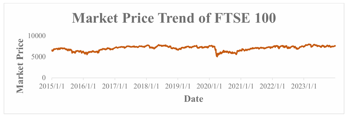
Figure 2: Market Price Trends of FTSE 100

Table 1 summarizes SP500 and FTSE 100 daily return descriptive information. These statistics provide significant information about time series data, which is needed to understand both indices' behavior during the given time period. Descriptive statistics are used to analyze the performance of financial institutions [11].

Table 1: Descriptive Statistics

The average daily return of the S&P 500 is 0.00037, whereas the median is 0.00056. This indicates that daily returns exhibit a slight positive bias. The SP500 exhibited moderately positive daily returns during the review period. The FTSE 100's average daily return is 0.00006. The mean and median differ, signifying a skewed distribution with a slight positive shift. The daily returns of the S&P 500 have a standard deviation of 0.01155, indicating mild activity volatility. The random sample's variance around the population mean is 0.00013. The standard deviation for the FTSE 100 is 0.01027, signifying that it exhibits less volatility than the S&P 500. The population and sample variances of 0.00011 indicate that the FTSE 100 had less return variability during the analyzed period, corroborating this result. The skewness of the SP500 is -0.80524, whereas that of the FTSE 100 is -0.87888. This indicates that both distributions exhibit left skewness, signifying that negative returns were more prevalent than positive ones during the observation period. The FTSE 100 demonstrated more pronounced negative returns than the S&P 500 owing to its negative skewness.

5.Analysis of Models

5.1.Analysis of the Autoregressive (AR) Model

The model equation that forecasts return on equity using an intercept and the product of a coefficient with the previous day return provides market behavior and information (See Table 2-5).

Table 2: Autoregressive (AR) Model Regression Analysis of SP500

Table 3: Autoregressive (AR) Model Coefficients of SP500

Table 4: Autoregressive (AR) Model Regression Analysis of FTSE 100

Table 5: Autoregressive (AR) Model Coefficients of FTSE 100

The SP500 intercept of 0.00043 predicts favorable returns, despite no changes from the previous day. The negative coefficient of -0.00034 indicates an indirect association between obesity and exercise. The negative coefficient suggests a weak mean reversion characteristic, meaning a portfolio with a favorable return today would likely have a slightly lower return tomorrow. Thus, previous performance has no effect on future returns, resulting in a zero anticipated return. This highlights the model's ability to maintain return estimates even if prior returns change.

Similar to FTSE, the intercept is 0.00008; due to a cautious market or less variation than SP500, FTSE has a lower baseline return expectation. The coefficient has a negative sign and a significantly greater negative value of -0.00279; this value suggests mean reversion is more precise since past returns are reversed faster in the succeeding period. The AR model's examination of the indices demonstrates that it can capture the intricate topography of financial time series, where historical returns temper future returns with a slight influence. These models prepare for more complex models like the Moving Average (MA) and ARMA models, which use prior errors to improve prediction accuracy.

5.2.Analysis of the Moving Average (MA) Model

The SP500 and FTSE 100 MA models answer problems like how past inaccuracy affects future performance. Since it estimates market returns, the MA model uses the mean return as its benchmark. SP500's mean return (μ) is 0.00037 with an intercept of 0.00043, and the lagged error coefficient is -0.00034. The negative sign implies that prior period mistakes effect current period returns in the reverse manner; if it overestimated returns, then it was somewhat corrected downward. In turbulent markets, this negative adjustment affects the predicted return, resulting in a more cautious milestone. The index is adjusted more negatively if the latest period return indicates a deviation from its predicted trend. This model's forecasted return for FTSE 100 is 0.00010, and for SP500 is 0.00043 (See Table 6-10).

The MA model shows that earlier errors affect return predictions, especially given financial markets' high-or-low volatility. Through application of these frameworks, SP500 and FTSE 100 have unique market behavior and structure that alter how errors are gauged to estimate future returns, increasing future forecasting.

Table 6: Moving Average (MA) Model Regression Analysis of SP500

Table 7: Moving Average (MA) Model Coefficients of FTSE 100

Table 8: Moving Average (MA) Forecast

Table 9: Moving Average (MA) Model Regression Analysis of FTSE 100

Table 10: Moving Average (MA) Model Coefficients of FTSE 100

5.3.Analysis of the Autoregressive Moving Average

For complicated and accurate forecasting, the ARMA model allows direct inclusion of historical returns and errors. It is ideal for financial time series analysis because it includes autoregressive (AR) to identify the influence of prior returns and moving average (MA) to control forecasting errors. The SP500 model Intercept is 0.00043, and the AR's coefficient is -0.00034. The FTSE100 index ARMA model uses a smaller intercept of 0.00007. The AR coefficient is -0.00278, which is larger than SP500, indicating that returns to mean following a high prior return are more likely than SP500 (See Table 11). The FTSE 100 is more likely to have negative anticipated returns.

Table 11: Autoregressive Moving Average

6.Conclusion

The objective of this paper was to evaluate time series models, such as auto regressive (AR), moving average (MA), and auto regressive moving average (ARMA), in response to the time series data of the SP500 and FTSE 100 index from 2015 to 2023. Furthermore, the analysis pinpointed the key differences between these indices and the predicted range of fluctuations and recoveries for each. SP500's volatility was higher than that of FTSE 100, which generally increased. The COVID-19 outbreak significantly impacted both of these indices during the initial half of the 2020 calendar year. However, the FTSE 100's recovery was significantly more rapid due to the stability of the companies that comprise this index. The AR model illustrated the correlation between historical and contemporary returns, and accordingly, neither index exhibited significant mean reversion. It implies that the returns of one day are not influenced by the returns of the following day, or, in other words, the performance of one day does not affect the performance of the next day. For the same reasons, the presence of negative second coefficients implies that high returns on one day typically result in slightly lower returns on the subsequent day. Conversely, the FTSE 100's market participants displayed more efficient corrective action, as evidenced by their elevated RMM values. However, the SP500 market also needed a longer period of time to recover.

Future research can concentrate on the comparison of the AR, MA, and ARMA models for a broader range of financial indicators, particularly those that are indicative of emerging or other highly unstable markets. The objective was to enhance the confidence in the adaptability of these models by stress-testing them in a variety of financial environments. Additionally, the accuracy of these models could be improved in the event of an unstable economic environment or a significant shift in market sentiment through the incorporation of external variables such as sentiment indices or geopolitical indicators. The utilization of machine learning methodologies in conjunction with other conventional time series models is an additional area that could be investigated in the future. This combination has the potential to enhance the models' capacity to detect complex patterns in markets and rail with high fluctuation, such as the 2008 financial collapse or COVID-19. Researchers and financial analysts can offer more precise predictions, which are particularly beneficial to investors and policymakers in the dynamic financial markets, by refining these models, which would necessitate the implementation of novel methodologies.

References

[1]. O’Hara, M. (2015). High frequency market microstructure. Journal of Financial Economics, 116(2), 257–270.
[2]. Brooks, C., & Hinich, M. J. (1999). Cross-correlations and cross-bicorrelations in Sterling exchange rates. Journal of Empirical Finance, 6(4), 385-404.
[3]. Chen, J. (2023). Analysis of bitcoin price prediction using machine learning. Journal of Risk and Financial Management, 16(1), 51
[4]. Choi, H., & Varian, H. (2012). Predicting the present with Google Trends. Economic record, 88, 2-9.
[5]. Kanade, V., Devikar, B., Phadatare, S., Munde, P., & Sonone, S. (2017). Stock market prediction: Using historical data analysis. International Journal of Advanced Research in Computer Science and Software Engineering, 7(1), 267-270.
[6]. Gomes, M. V., & Cicogna, M. P. V. (2023). S&P500 volatility and Brexit contagion. Gestão & Produção, 30, e8422.
[7]. Madaleno, M., & Pinho, C. (2012). International stock market indices comovements: a new look. International Journal of Finance & Economics, 17(1), 89-102.
[8]. Kaya, P., & Güloğlu, B. (2017). Modeling and Forecasting the Markets Volatility and VaR Dynamics of Commodity. BDDK Bankacılık ve Finansal Piyasalar Dergisi, 11(1), 9-49.
[9]. Pappas, S. S., Ekonomou, L., Karamousantas, D. C., Chatzarakis, G. E., Katsikas, S. K., & Liatsis, P. (2008). Electricity demand loads modeling using AutoRegressive Moving Average (ARMA) models. Energy, 33(9), 1353-1360.
[10]. Jamaludin, A. R., Yusof, F., Kane, I. L., & Norrulasikin, S. M. (2016). A comparative study between conventional ARMA and Fourier ARMA in modeling and forecasting wind speed data. In AIP Conference Proceedings (Vol. 1750, No. 1). AIP Publishing.
[11]. Shukla, P. J. (2024). AN ANALYSIS OF FINANCIAL PERFORMANCE OF INFOSYS & WIPRO USING DESCRIPTIVE STATISTICS: DURING 2017-18 TO 2021-22. Journal of Capital Market and Securities Law, 7(1), 30-34.
Cite this article
Zeng,W. (2024). Application of AR, MA, and ARMA Models in Financial Time Series Analysis. Advances in Economics, Management and Political Sciences,141,177-184.
Data availability
The datasets used and/or analyzed during the current study will be available from the authors upon reasonable request.
Disclaimer/Publisher's Note
The statements, opinions and data contained in all publications are solely those of the individual author(s) and contributor(s) and not of EWA Publishing and/or the editor(s). EWA Publishing and/or the editor(s) disclaim responsibility for any injury to people or property resulting from any ideas, methods, instructions or products referred to in the content.
About volume
Volume title: Proceedings of ICFTBA 2024 Workshop: Finance's Role in the Just Transition
© 2024 by the author(s). Licensee EWA Publishing, Oxford, UK. This article is an open access article distributed under the terms and
conditions of the Creative Commons Attribution (CC BY) license. Authors who
publish this series agree to the following terms:
1. Authors retain copyright and grant the series right of first publication with the work simultaneously licensed under a Creative Commons
Attribution License that allows others to share the work with an acknowledgment of the work's authorship and initial publication in this
series.
2. Authors are able to enter into separate, additional contractual arrangements for the non-exclusive distribution of the series's published
version of the work (e.g., post it to an institutional repository or publish it in a book), with an acknowledgment of its initial
publication in this series.
3. Authors are permitted and encouraged to post their work online (e.g., in institutional repositories or on their website) prior to and
during the submission process, as it can lead to productive exchanges, as well as earlier and greater citation of published work (See
Open access policy for details).