1. Introduction

Volatility is an essential measure of risk in financial markets. It measures the extent of variation, i.e., the magnitude of deviation of prices in an asset over time. Volatility is about the uncertainty of the market based on new economic scenarios and investor sentiment. Given the recent extreme swings in financial assets, it has become increasingly relevant—especially for digital assets and technology stocks. Accurate modelling of volatility is important for risk management and regulatory compliance [1].

Financial time series exhibit volatility clustering—high or low volatilities beget further such periods [2]. This property makes the traditional models inadequate to model volatility dynamics. For this reason, models such as the Generalised Autoregressive Conditional Heteroskedasticity (GARCH) have been developed to improve the forecasting of volatility [3]. They also can deal with mean-reverting traits that variable asset classes usually experience. It is important for investors and analysts to have such an analysis of volatility. The volatilities of various asset classes will give us a better understanding of market dynamics, thereby reducing risk [4].

This paper will focus on the volatility of Bitcoin (BTC-USD) and MicroStrategy (MSTR). Bitcoin is the highest valued cryptocurrency; its price is highly volatile. That said, MicroStrategy's more precarious position is a function of the fact that its stock is essentially tied to Bitcoin because it holds so much. The paper analyses the volatility patterns of both assets. It studies how Bitcoin’s volatility affects corporate equity exposed to it. It also explores the broader implications for financial markets.

2. Literature Review

Researchers found that price changes tended to be followed by further large changes at different scales, leading to the discovery of volatility clustering [2][5]. This realisation paved the way for the construction of contemporary volatility models, particularly ARCH and GARCH [3][6]. Since these models account for time-varying factors, they can yield improved predictions of volatility. The GARCH(1,1) model is well established in financial econometric literature primarily because the model allows for straightforward identification of volatility clustering. The importance of this invention in volatile financial modelling was clearly pointed out by Engle, as it can capture transitory shocks and long-term volatility persistence [1]. GARCH models have since then been used to model volatility in both traditional and emerging financial markets [7].

Significant financial events often have the propensity to cause increased volatility within global marketplaces. The 2008 Global Financial Crisis witnessed some massive volatility surges—Volatility being represented by indices like VIX [8]. Research using the GARCH model showed that this event introduced stock market uncertainty and panic in systems successively, which keeps long-range volatility dependence continued [9]. Likewise in the field, as in COVID-19 fell due to economic instability, which massively layered on price volatility. Along these lines, empirical studies found that while the turbulence shocks were immediate, in many of the most globally interconnected markets they also remained persistent [10].

Cryptocurrencies, especially Bitcoin, are key in volatility studies. Bitcoin’s volatility is much higher than traditional assets due to its speculative nature [11]. It experiences long high-risk periods, followed by short stabilisation phases [7]. This makes Bitcoin perfect for studying volatility, especially during major financial or macroeconomic events.

In recent years, companies like MicroStrategy and Tesla have adopted Bitcoin as part of their treasury strategy, introducing new layers of volatility to traditional equities. MicroStrategy’s large Bitcoin holdings have made its stock increasingly susceptible to the same volatility patterns observed in the cryptocurrency market. While limited literature has specifically addressed the volatility relations of Bitcoin and corporate equities, the relationship between digital assets and traditional markets is an emerging area of study. The role of Bitcoin was examined as a hedge or safe haven in global equity markets, finding that Bitcoin exhibits properties that are distinct from traditional assets, yet its volatility remains a risk factor for firms exposed to it [12].

3. Data

3.1. Data Collection

The data for this study was sourced from Yahoo Finance and consists of daily closing prices for Bitcoin (BTC-USD) and MicroStrategy (MSTR) from September 1, 2019, to September 1, 2024. The dataset was cleaned to focus on the close prices, which were used to compute log returns for further statistical analysis. Figure 1 and Figure 2 depict the daily closing prices of Bitcoin and MicroStrategy, highlighting key periods of volatility between September 2019 and September 2024. The Bitcoin graph shows significant price movements, including the notable bull run in 2021. Similarly, the MicroStrategy graph reveals the close relationship between its stock performance and Bitcoin’s price, as the company holds substantial Bitcoin assets. This relationship can be seen whenever there is a significant fluctuation in the cryptocurrency market. The returns of the two underlyings have been computed, and the statistics are shown in Table 1.

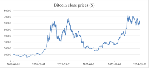
Figure 1: Historical Close Prices of Bitcoin (BTC-USD)

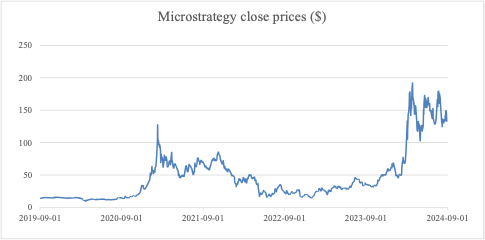
Figure 2: Historical Close Prices of MicroStrategy (MSTR)

Table 1: Statistical Summary

3.2. Autocorrelation

In this section, an autocorrelation test is conducted using the Autocorrelation Function (ACF) and Partial Autocorrelation Function (PACF) (See Figure 3 and Figure 4). Each of these is done to see if past values of returns are related to future values. The ACF provides insights into the correlation of log returns with their lagged values, while the PACF helps in deciding how many lags are significant, as it removes the correlations explained by previous lags. These tests are important for assessing the suitability of GARCH, as they verify whether log returns show autocorrelation, which usually indicates the presence of volatility clustering—a key characteristic in financial time series.

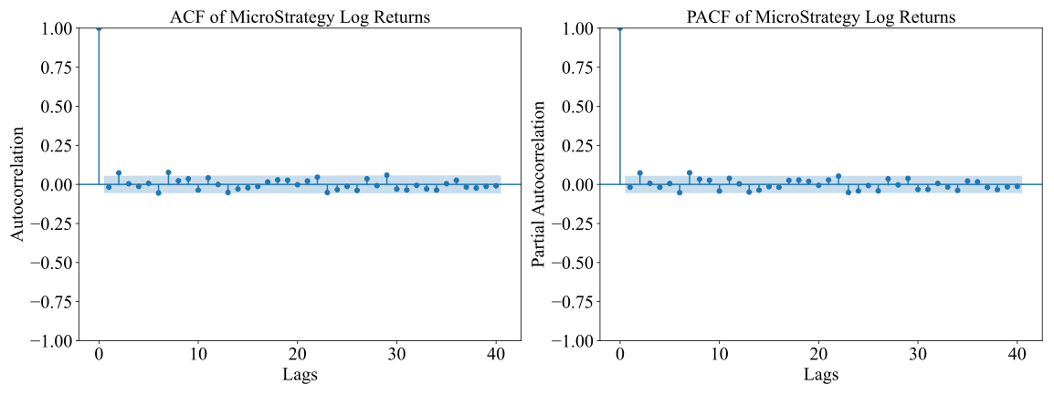
Figure 3: ACF and PACF for Bitcoin returns

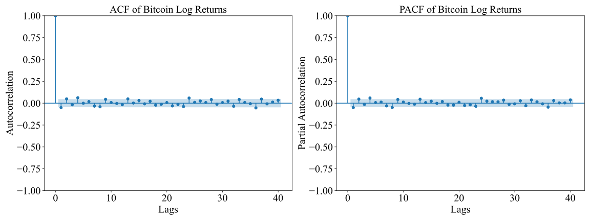
Figure 4: ACF and PACF for MicroStrategy returns

The obtained autocorrelation results for Bitcoin and MicroStrategy log returns were insignificant beyond the first lag. The returns have short-term dependencies, but this outcome suggests they are mostly random, with no strong autocorrelations beyond the initial period, which is typical for financial return data. Normally, such data shows low levels of autocorrelation at higher lags. By analyzing the ACF and PACF plots for both assets, it is evident that most of the autocorrelations fall within the confidence intervals, confirming that the series behaves like a random walk with minor dependencies. This supports the assumption of the GARCH model, which accounts for volatility clustering but does not rely on strong autocorrelation in returns.

3.3. ADF Test

With Python, this paper performed the ADF test to check stationarity for two series: Bitcoin and MicroStrategy. Stationarity is one of the most desirable features, indicating that the statistical properties of the data, such as mean and variance, remain constant over time. Hence, it provides a solid foundation for further analysis. The results of the ADF test are presented in Table 2.

Table 2: ADF Test Results

The ADF tests for the log return of Bitcoin and MicroStrategy confirm that the log returns are stationary. This is indicated by the rejection of the null hypothesis of a unit root in both time series, where the test statistics are more negative than the critical values at standard significance levels. The stationarity of the log returns ensures that the key condition for applying GARCH models is met.

4. Methodology

The methodology section now describes how volatility for Bitcoin and MicroStrategy is analysed through the GARCH(1,1) model. This paper first specify the GARCH(1,1) model in detail, focusing on how its autoregressive and moving average components capture time-varying volatility. Estimation will involve using maximum likelihood estimation (MLE) to fit the model to the log returns of both assets. Finally, this paper introduces the model diagnostics approach, including residual analysis and statistical tests, which allows us to check the appropriateness of the model for data. This section describes the procedure for implementing the model without presenting the actual results.

4.1. GARCH(1,1) Model Specification

Bollerslev presented GARCH in 1986. It generalises the ARCH model, which Engle introduced in 1982 [3][6]. This model adds autoregressive and moving average parts of volatility. It is well-suited for financial time series, which often have volatility clustering. In GARCH(1,1), the conditional variance \( σ_{t}^{2} \) at time t is modelled based on the last squared residual and conditional variance.

Where \( σ_{t}^{2} \) denotes the conditional variance, \( ϵ_{t-1}^{2} \) is the lagged squared error term (or residual), and \( σ_{t-1}^{2} \) is the lagged conditional variance. The parameters \( {α_{1}} \) and \( {β_{1}} \) capture the short-term impact of shocks and the persistence of volatility respectively [1]. Given the patterns of Bitcoin and MicroStrategy, the GARCH(1,1) model is an ideal choice. Its flexibility makes it useful when learning how Bitcoin’s price fluctuations may influence MicroStrategy’s stock.

4.2. Estimation Process

The GARCH model parameters were estimated using MLE, which is a standard approach in financial econometrics to model fluctuating volatility [13]. MLE identifies parameters that best fit the observed data. This was done using the arch package in Python, designed for fitting GARCH models to single time series.

MLE is advantageous because it yields unbiased and consistent estimates. The parameters include \( {α_{0}} \) (the constant term), \( {α_{1}} \) ​ (the coefficient for the last squared shock), and \( {β_{1}} \) ​ (the coefficient for the last volatility). The significance of both \( {α_{1}} \) and \( {β_{1}} \) ​ indicates whether volatility shocks are temporary or long-term. This is key for assets like Bitcoin, where sudden market shifts can cause large and lasting volatility changes.

4.3. Model Diagnostics

Diagnostic checks are crucial to check the accuracy and robustness of the model. First, residual analysis is conducted to ensure that they are normally distributed and independent. Next, the Ljung-Box Q-test is applied to check for any remaining autocorrelation. This paper looks for a high p-value from this test to ensure no conditional heteroskedasticity remains. Then, the ARCH test is performed to ensure no conditional heteroskedasticity remains.

5. Results

5.1. GARCH(1,1) Model Results for Bitcoin

The results highlight the significance of the model’s parameters in capturing the time-varying nature of Bitcoin’s volatility. In particular, the coefficients offer insights into the persistence of volatility. Table 3 summarises these findings.

Table 3: Bitcoin GARCH(1,1) Model

As displayed in Table 3, the \( {α_{0}} \) parameter, which represents the baseline level of volatility, is relatively low at 6.7558e-05. This indicates that Bitcoin’s intrinsic, or unconditional, volatility is quite small. However, more emphasis should be placed on the alpha ( \( {α_{1}} \) ) and beta ( \( {β_{1}} \) ) coefficients, which describe how recent shocks and past volatility affect future volatility.

For Bitcoin, \( {α_{1}} \) is 0.1237, indicating that recent shocks to the system have a moderate effect on volatility. This shows that Bitcoin does not overreact to individual market shocks. However, β1, the coefficient measuring the persistence of volatility over time, is 0.8357, reflecting the long-lasting nature of volatility. When summing the values of \( {α_{1}} \) and \( {β_{1}} \) ( \( {α_{1}} \) + \( {β_{1}} \) = 0.9594), it suggests that nearly 96% of the volatility is carried over from one period to the next, meaning volatility shocks in Bitcoin tend to have a prolonged effect. This high persistence is typical of financial time series, especially for assets like Bitcoin, which are known for periods of high volatility followed by further clusters of high volatility.

5.2. GARCH(1,1) Model Results for MicroStrategy

For MicroStrategy, the GARCH(1,1) model estimation provides valuable insights into the volatility dynamics of its stock returns. Table 4 presents the key parameters for both the mean and volatility models.

Table 4: MicroStrategy GARCH(1,1) Model

Similar to Bitcoin, the GARCH(1,1) model for MicroStrategy provides insights into the conditional volatility of its stock returns. Table 4 shows that \( {α_{0}} \) for MicroStrategy is slightly lower at 6.1279e-05, indicating a low baseline level of volatility. The alpha ( \( {α_{1}} \) ) coefficient for MicroStrategy is 0.1000, suggesting that recent market shocks also have a moderate effect on its volatility, slightly less than the effect seen for Bitcoin.

Accordingly, the beta ( \( {β_{1}} \) ) for MicroStrategy is even higher at 0.8800, suggesting that past volatility plays an even larger role in determining current volatility. The summation of \( {α_{1}} \) and \( {β_{1}} \) for MicroStrategy reaches 0.9800, indicating that 98% of volatility is carried over to the next period. This means that volatility only slowly dissipates in MicroStrategy and cannot be solely attributed to Bitcoin’s influence. Additional factors, such as company-specific events and broader equity market trends, also play a role.

5.3. Graphical Analysis

The estimates allow us to observe the patterns in time-varying volatility and investigate the correlation between the two assets. The periods of high volatility in both assets are typically driven by market events, macroeconomic factors, and Bitcoin-specific fluctuations. Figure 5 and Figure 6 show the conditional volatility estimates for Bitcoin and MicroStrategy.

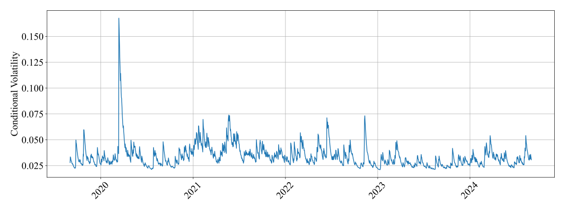
Figure 5: Bitcoin (BTC-USD) Conditional Volatility-GARCH(1,1)

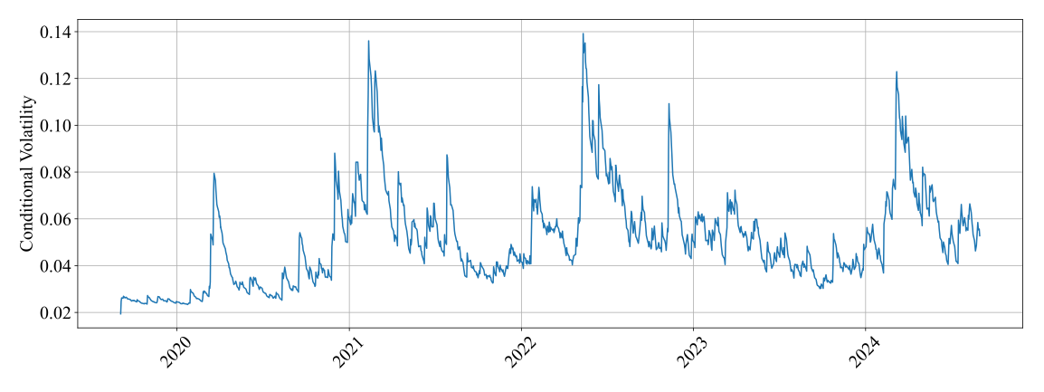
Figure 6: MicroStrategy (MSTR) Conditional Volatility-GARCH(1,1)

The GARCH results clearly provide evidence of the strong relationship between Bitcoin and MicroStrategy in terms of their volatility dynamics. This is unsurprising, given that MicroStrategy holds a substantial amount of Bitcoin, making its volatility patterns closely aligned with Bitcoin’s. The sum of \( {α_{1}} \) and \( {β_{1}} \) for both assets is very close to 1, indicating that volatility shocks are persistent and exhibit volatility clustering over time. In this regard, a graphical analysis of Bitcoin and MicroStrategy’s conditional volatility offers a more intuitive understanding of their relationship.

5.3.1. COVID-19 Period (March to June 2020)

At the onset of the COVID-19 pandemic in March 2020, global markets faced extreme uncertainty, which triggered significant volatility across asset classes. Bitcoin’s price dropped sharply from around $9,000 in early March to below $5,000 by mid-March as investors sought liquidity during the financial crisis. However, Bitcoin rebounded quickly as the market stabilised, fueled by speculative interest and rising demand for alternative assets. This led to increased volatility, as reflected in the GARCH model, with notable spikes throughout the remainder of 2020.

During this time, MicroStrategy had not yet begun its Bitcoin acquisition strategy, so its stock volatility was driven more by macroeconomic factors affecting the broader equity and tech sectors. As a result, there was minimal correlation between Bitcoin and MicroStrategy’s volatility. The tech market crash during the COVID-19 period influenced MicroStrategy’s stock performance, but without any direct connection to Bitcoin, the two assets were largely independent in their volatility patterns.

5.3.2. 2022 to Early 2023 Period

By 2022, Bitcoin and MicroStrategy had indeed seen their relationship radically change, largely due to the introduction of Bitcoin into one of MicroStrategy’s critical corporate strategies. Back in August 2020, MicroStrategy did a big community announcement regarding its Bitcoin purchase of 21,454 BTC for $250 million, explaining that it had bought Bitcoin as a hedge against inflation, which it considered a better store of value than cash. As time advanced, however, MicroStrategy’s Bitcoin acquiring program typically continued, and the company bought more Bitcoin, especially at discounted prices, leading to the holding of a significant amount of Bitcoin on its balance sheet.

The period witnessed the highest volatility in the crypto market, ever since the FTX collapse in late 2022, from which the market has yet to fully recover. The FTX bankruptcy set off a chain reaction that triggered a massive sell-off across other markets as well, and Bitcoin’s price subsequently fell from approximately $47,000 early in 2022 to below $17,000 by the end of the year. Also, there were more regulations, traders not believing, and more fears that the previous pandemic would return, making Bitcoin sink and adding to the already existent volatility.

This excess volatility, for MicroStrategy, was attributed to its Bitcoin position. Investors utilised MicroStrategy as a means of investment in Bitcoin, so that, when the price of Bitcoin fell, concerns about the company’s financial stability went up too, and these fears made stock price caustics even worse. The GARCH model goes on to unravel the commonality in spikes where the increases in volatility change co-movements of Bitcoin and MicroStrategy as the situation demands. Bitcoin going down in the market, compounded by macroeconomic factors like rising interest rates and concerns of recession, were the last drops that sealed the fate of both.

5.3.3. Early 2024 Period

A comeback of Bitcoin initiated a wave in the beginning of 2024. Institutional interest was rekindled, regulatory clarity enhanced, and new financial products came into existence. This prompted a turnaround in the market as investors began to believe in the potential of digital assets, and ETFs generally stabilised it. Speculative trading increased as prices rose from 2022 lows, exacerbating price volatility. Over in the stock market, MicroStrategy has seen a recovery too. The largest corporate holder of Bitcoin, its fortunes were linked to the cryptocurrency. As investors started to view the company’s performance as a Bitcoin proxy, the prices began moving in parallel. During the rally, the GARCH model showed a very strong correlation.

Institutional players drove this comeback. Large investors flooded back, ramping up demand and intensifying volatility for both assets. MicroStrategy’s stock rode Bitcoin's waves, its fate inexorably linked to the digital currency's market trends. This symbiotic relationship defined the period, with each uptick in Bitcoin reverberating through MicroStrategy’s valuation.

6. Conclusion

In this study, the GARCH(1,1) model was applied to examine the volatility patterns of both Bitcoin and MicroStrategy. The analysis revealed significant volatility persistence in both assets, where past price shocks continue to influence future price movements. Bitcoin’s volatility is largely driven by speculation, debates over block size, regulatory changes, monetary policy announcements, and broader economic factors, all of which contribute to its frequent and dramatic price swings. This strong volatility clustering is a defining characteristic of Bitcoin.

MicroStrategy, due to its substantial Bitcoin holdings, exhibited volatility patterns closely mirroring those of Bitcoin, particularly during periods of market stress. The model highlighted several key events that triggered spikes in volatility for both assets, such as the collapse of FTX in early 2022, Bitcoin’s subsequent rally, and the financial uncertainty during the COVID-19 pandemic. These incidents demonstrated a closer correlation between Bitcoin and MicroStrategy’s stock, especially as MicroStrategy’s exposure to Bitcoin made its equity more sensitive to Bitcoin’s price movements.

In summary, this research underscores the significant risks associated with corporate holdings in digital currencies like Bitcoin. The integration of digital assets into corporate portfolios, as seen with MicroStrategy’s significant Bitcoin holdings, highlights a shifting paradigm in market behavior. Traditional models of risk and volatility are being challenged by the increasing influence of cryptocurrencies on corporate equities. This study shows how companies exposed to digital currencies could be subject to the significant volatility that is independent from the company's core business. Navigating a more connected financial ecosystem is becoming more challenging as the volatility of digital assets impacts the performance of individualised stocks and drives through entire market systems.

References

[1]. Engle, R. F. (2001). GARCH 101: The use of ARCH/GARCH models in applied econometrics. Journal of Economic Perspectives, 15(4), 157-168.
[2]. Mandelbrot, B. (1963). The variation of certain speculative prices. Journal of Business, 36(4), 394-419.
[3]. Bollerslev, T. (1986). Generalized autoregressive conditional heteroskedasticity. Journal of Econometrics, 31(3), 307-327.
[4]. Poon, S. H., & Granger, C. W. J. (2003). Forecasting volatility in financial markets: A review. Journal of Economic Literature, 41(2), 478-539.
[5]. Fama, E. F. (1965). The behavior of stock-market prices. The Journal of Business, 38(1), 34-105.
[6]. Engle, R. F. (1982). Autoregressive conditional heteroskedasticity with estimates of the variance of United Kingdom inflation. Econometrica, 50(4), 987-1007.
[7]. Baur, D. G., & Dimpfl, T. (2018). The volatility of Bitcoin and its role as a hedge in global markets. Journal of Economic Behavior & Organization, 149, 52-69.
[8]. Whaley, R. E. (2009). Understanding the VIX. Journal of Portfolio Management, 35(3), 98-105.
[9]. Zivot, E. (2009). Practical issues in the analysis of univariate GARCH models. In Routledge Handbook of Econometrics (Vol. 1, pp. 113-155).
[10]. Zhang, D., Hu, M., & Ji, Q. (2020). Financial markets under the global pandemic of COVID-19. Finance Research Letters, 36, 101528.
[11]. Cheah, E.-T., & Fry, J. (2015). Speculative bubbles in Bitcoin markets? An empirical investigation into the fundamental value of Bitcoin. Economics Letters, 130, 32-36.
[12]. Bouri, E., Molnár, P., Azzi, G., Roubaud, D., & Hagfors, L. I. (2017). On the hedge and safe haven properties of Bitcoin: Is it really more than a diversifier? Finance Research Letters, 20, 192-198.
[13]. Harvey, A. C. (1990). Forecasting, structural time series models and the Kalman filter. Cambridge University Press.
Cite this article
Ma,H. (2025). Volatility Dynamics Analysis of Bitcoin (BTC-USD) and MicroStrategy (MSTR). Advances in Economics, Management and Political Sciences,145,190-199.
Data availability
The datasets used and/or analyzed during the current study will be available from the authors upon reasonable request.
Disclaimer/Publisher's Note
The statements, opinions and data contained in all publications are solely those of the individual author(s) and contributor(s) and not of EWA Publishing and/or the editor(s). EWA Publishing and/or the editor(s) disclaim responsibility for any injury to people or property resulting from any ideas, methods, instructions or products referred to in the content.
About volume
Volume title: Proceedings of ICFTBA 2024 Workshop: Human Capital Management in a Post-Covid World: Emerging Trends and Workplace Strategies
© 2024 by the author(s). Licensee EWA Publishing, Oxford, UK. This article is an open access article distributed under the terms and
conditions of the Creative Commons Attribution (CC BY) license. Authors who
publish this series agree to the following terms:
1. Authors retain copyright and grant the series right of first publication with the work simultaneously licensed under a Creative Commons
Attribution License that allows others to share the work with an acknowledgment of the work's authorship and initial publication in this
series.
2. Authors are able to enter into separate, additional contractual arrangements for the non-exclusive distribution of the series's published
version of the work (e.g., post it to an institutional repository or publish it in a book), with an acknowledgment of its initial
publication in this series.
3. Authors are permitted and encouraged to post their work online (e.g., in institutional repositories or on their website) prior to and
during the submission process, as it can lead to productive exchanges, as well as earlier and greater citation of published work (See
Open access policy for details).