1. Introduction

In data science and statistics, time series forecasting is a substantial area of research. It is widely used in finance, economics, meteorology, and engineering. Time series data distinguished by a sequential arrangement of data points, is a critical capability in various industries, as it allows for the prediction of future values. In order to address this challenge, researchers and practitioners have devised a diverse array of time series modelling methodologies. Two well-known and frequently employed statistical methods are the ARIMA and ETS models.

In addition to seasonality and non-stationarity, trends in the data introduce an additional layer of complexity to time series forecasting. The ARIMA model utilises autoregressive and moving average components, as well as differencing, to capture linear relationships and account for non-stationarity. The complexity of seasonal patterns may continue to pose a challenge, despite ARIMA's adaptability. Frequently, the ETS model yields superior results than ARIMA when applied to time series data that exhibit robust seasonal patterns, due to its explicit accounting of error, trend, and seasonality. This is because it is ideal for predicting demand and sales during specific seasons.

The ARIMA and ETS models have been the subject of numerous recent comparisons. Despite ARIMA's reputation for adaptability, ETS outperforms ARIMA in time series data with significant seasonality [1]. Kazemi confirmed that ETS is particularly adept at capturing fleeting seasonal variations [2]. Selamlar's criteria for model selection emphasise the importance of ensuring that the model is well-suited to the distinctive characteristics of the time series [3].

The decision between ARIMA and ETS is still dependent on certain information properties and application situations, even though there are existing comparisons. The purpose of this paper is to empirically assess these models across a wide range of datasets in order to improve understanding of their relative efficacy. The study contributes through empirically analyzing actual data to assess the performance of the models and providing recommendations for selecting suitable forecasting models based on specific time series features.

2. Models Comparisons

The comparison between ARIMA and ETS models are through two datasets from the fpp2 package in R, which is Forecasting: Principles and Practice (2nd ed) [4]. GooG (Google stock prices, non-seasonal data) and Arrivals (Australian tourism arrivals, seasonal data) are chosen as the examples for two different cases of Seasonality. The performance of these models in capturing the underlying patterns of both datasets will be assessed, while their respective strengths will be discussed.

2.1. Non-Seasonal Sample: Google Stock Prices (GooG)

The daily closing prices of Google stock are included in the GooG dataset. ARIMA modelling is a well-known method for effectively managing linear trends and non-stationary data, and this time series is non-seasonal, rendering it an ideal candidate.

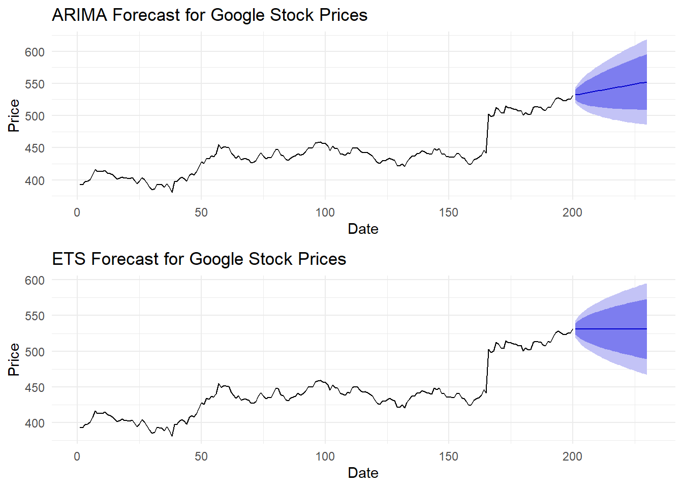
Figure 1: The prediction of Google Stock Price through ARIMA and ETS.

Figure 1 shows the forecasts for Google stock prices using the ARIMA and ETS models, each with their respective 80% and 95% confidence intervals. The selected ARIMA model for modelling the prices of Google stock is ARIMA (1,1,0). This model accurately captures the general pattern in the data and extrapolates it to make predictions for the future. The upper plot showcases the model's proficiency in producing precise predictions. However, the elongated confidence intervals suggest that uncertainty is increasing as time progresses. The ETS model forecast is shown in the lower plot. The ETS model, similar to the ARIMA model, also contains the trends. Nevertheless, the model's ability to accurately represent seasonal components is limited by the absence of pronounced seasonal patterns in the data. The ETS model and the ARIMA model produce forecasts that closely align with the trend observed in the historical data.

Ultimately, both models produce comparable predictions, although ARIMA may have a slight advantage in terms of its ability to adapt to the non-seasonal features of the data. Still, the expanding confidence intervals in both models emphasize the growing ambiguity when making predictions over extended time periods, which is a typical characteristic in time series forecasting.

2.2. Seasonal Sample: Australian Tourism Arrivals (Arrivals)

The Arrivals dataset comprises quarterly data regarding the quantity of international tourists visiting Australia. This time series demonstrates noticeable seasonal patterns, indicating that it is well-suited for the ETS model, which explicitly incorporates seasonality into its modeling.

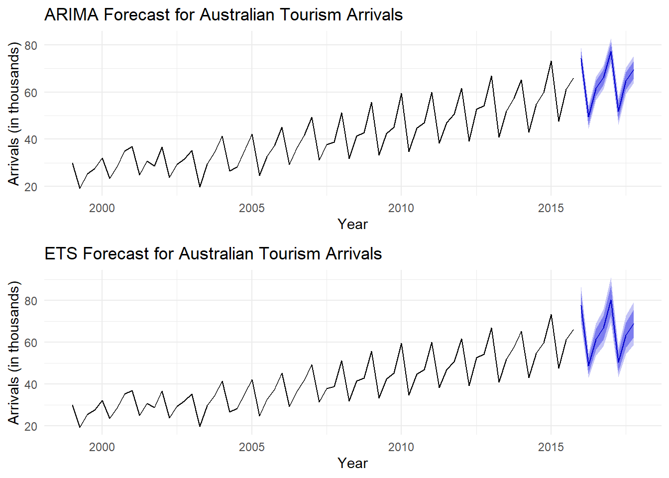
Figure 2: The prediction of Australian Tourism Arrivals through ARIMA and ETS.

Figure 2 shows the tourist arrival forecasts for Australia using both ARIMA and ETS models, which share the same confidence intervals. The first graph presents the ARIMA model's forecast, effectively reflecting the overall data trend and incorporating seasonal differencing for seasonality. However, it struggles to replicate the historical seasonal peaks and troughs accurately. The widening confidence intervals over time highlight growing uncertainty, particularly for seasonal fluctuations.

The ETS model effectively analyzes time series data with clear trend and seasonal patterns, capturing the seasonal fluctuations in Australian tourism arrivals and yielding forecasts that align well with historical cycles. Its confidence intervals exhibit stability and reduced widening, indicating that the ETS model provides reliable forecasts for this seasonal data.

Although both models can predict the general trend, the ETS model exhibits a more robust capability to accurately represent the seasonal patterns present in the tourism arrivals data. ETS is the more appropriate option for data that exhibits robust and consistent seasonal patterns, such as the influx of Australian tourism arrivals. The comparison emphasizes the significance of choosing a model that corresponds to the particular attributes of the time series data. The ETS model's explicit treatment of seasonality in this dataset yields a forecast that is more precise and dependable.

3. Case Studies and Application Scenarios

3.1. Application Scenarios

(1) Seasonal Demand Forecasting: The ETS model is highly effective in forecasting sales for seasonal products, including winter clothing. Retailers are able to effectively manage inventory and minimize stockouts during periods of high demand by having the ability to accurately capture distinct seasonal patterns [5].

(2) Financial Time Series Forecasting: ARIMA is a widely-used model in financial markets, particularly for the prediction of stock prices or exchange rates. It is the preferred choice in this domain due to its exceptional ability to model non-stationary data with trends [6].

(3) Public Health Monitoring: ARIMA models can be useful for monitoring the spread of diseases with unpredictable patterns, such as influenza. Conversely, ETS models are more appropriate for predicting diseases that exhibit distinct seasonal patterns, which in turn facilitates preparedness during peak periods [1].

(4) Energy Consumption Forecasting: Energy companies frequently utilize ARIMA models to forecast overall consumption trends, while ETS models are employed when energy usage exhibits consistent seasonal patterns, such as heightened demand during winter months [7].

3.2. Case Studies

(1) Retail Sales Forecasting: In order to enhance inventory management and mitigate stockouts during peak seasons, a substantial retail chain implemented the ETS model to precisely predict seasonal product sales [5].

(2) Stock Price Prediction: The ARIMA model was successfully implemented by a financial institution to forecast the stock prices of a significant technology business. This approach was able to capture a robust non-stationary trend and generate dependable short-term predictions [7].

(3) Influenza Monitoring: The spread of influenza was monitored using both ARIMA and ETS models in a public health project. ETS accurately predicted seasonal peaks, facilitating effective preparation for flu seasons, while ARIMA captured the unpredictable nature of the disease's spread [1].

(4) Energy Consumption Forecasting: A utility company employed both ARIMA and ETS models to predict forthcoming energy demand. The ARIMA model was used to address the general upward trend, while the ETS model captured the seasonal fluctuations, enabling the company to optimize the allocation of resources [7].

4. Results and Discussion

4.1. Results

Two datasets were subjected to the ARIMA and ETS models: Australian Tourism Arrivals (Arrivals) and Google Stock Prices (GooG). The following is a summary of the model's performance on these datasets.

(1) Google Stock Prices (Non-Seasonal Data): The ARIMA model that was chosen for this dataset was ARIMA (1,1,0), which exhibited a satisfactory fit with the observed data. The forecasted values were in close alignment with the actual historical trends, demonstrating a high degree of accuracy in capturing the linear patterns evident in the data. This outcome is in accordance with the findings of Makridakis and Hibon, who observed that ARIMA is particularly effective in the modelling of linear trends and non-stationary data, notably in financial time series [7]. Taylor and Letham's research on scalable forecasting techniques further substantiates the efficacy of ARIMA in managing non-seasonal financial data [8]. Although the ETS model was typically effective, it produced slightly less accurate forecasts than ARIMA as a result of the absence of seasonal components in the Google Stock Prices data. This observation is consistent with the findings of Hyndman et al., who suggested that ETS models may not perform as well in non-seasonal contexts [9]. Nevertheless, Holt's fundamental research on exponential averaging serves as a foundation for comprehending the ETS model's inherent strengths in other contexts [10]. Typical of time series forecasting, the confidence intervals for both models widened over time, reflecting increased uncertainty as the forecasting horizon extended, as discussed by De Livera et al. [5].

(2) Tourist Arrivals in Australia (Seasonal Data): The ETS model was particularly adept at capturing the cyclical peaks and troughs of visitor arrivals, resulting in dependable forecasts that closely resembled historical seasonal patterns. This is in accordance with the results of Hyndman et al., who illustrated the model's exceptional ability to forecast seasonal time series [9]. Furthermore, Kourentzes, Petropoulos, and Trapero's investigation into the estimation of time series components across numerous frequencies offers additional evidence of the complexity of seasonal data that ETS models can handle [11].The ARIMA model, despite utilising seasonal differencing (SARIMA), was unable to accurately replicate the regular seasonal fluctuations to the same extent as the ETS model. This discovery is corroborated by Pankratz, who identified ARIMA's constraints in managing intricate seasonal patterns in the absence of additional model improvements [12]. Moreover, the difficulties ARIMA encounters in capturing the complex seasonal variations in health-related data are underscored by Petropoulos and Makridakis's research on COVID-19 forecasting [13]. Makridakis and Hibon previously observed that the ARIMA model's limitations in this context were emphasised by the more pronounced widening of confidence intervals, particularly in relation to seasonal variations [7].

These results suggest that the efficacy of both models is contingent upon the specific characteristics of the time series data, despite the fact that they are both effective.

4.2. Discussion

The ARIMA and ETS models' comparative analysis provides critical insights into their respective strengths and limitations:

Firstly, it is the suitability of the model. The ARIMA model is particularly well-suited for linear time series data and non-seasonal data, as evidenced by its robust performance with the Google Stock Prices dataset. This is in accordance with the fundamental research of Box and Jenkins, who demonstrated the effectiveness of ARIMA in modelling non-stationary data [6]. Furthermore, the practicality of ARIMA in financial market applications is emphasised by Taylor and Letham's research on forecasting at scale [8]. In contrast, the ETS model is particularly effective for time series that have significant seasonal components, such as the Australian Tourism Arrivals data. The model's capacity to expressly account for error, trend, and seasonality allows it to more effectively manage data with predictable seasonal patterns, as demonstrated by Hyndman and Athanasopoulos and further elaborated upon by Kourentzes et al. in their study on multiple frequencies [4, 11].

Additionally, it is evident that forecast accuracy and uncertainty comprise a substantial portion of the influence factors. The significance of selecting the appropriate model based on the specific attributes of the time series data is emphasised in the study. ETS offers more dependable forecasts in seasonal contexts, while ARIMA offers a more precise fit in non-seasonal contexts. This observation is consistent with the exhaustive comparison of forecasting methods by Makridakis and Hibon and is further supported by Holt's research on exponential smoothing [7, 10]. The increasing uncertainty in long-term predictions is underscored by the expanding confidence intervals in both models as the forecasting horizon lengthens. This phenomenon has been extensively examined by De Livera et al. [9] and observed in pandemic-related forecasting by Petropoulos and Makridakis [13].

In addition, it is apparent from the Practical Implications. The results underscore the importance of meticulously evaluating the fundamental data patterns when selecting a forecasting model for practitioners. The ETS model should be prioritised in situations where the data demonstrates distinct seasonal patterns. Conversely, ARIMA is a superior option for datasets in which seasonality is either absent or less pronounced, as observed by Seba et al. [1]. In cases involving complex seasonal patterns or multiple frequencies, Kourentzes et al.'s research also supports the use of ETS [11]. The specific application domain should also be taken into account when selecting between ARIMA and ETS. ARIMA may provide superior predictive performance in financial markets where trends are more prevalent than seasonality. Conversely, Kazemi [2] posits that industries like retail, which are characterised by seasonal demand, may derive greater advantages from ETS models.

5. Conclusion

This study offers a comparative examination of the ARIMA and ETS models in the context of time series forecasting, with a particular emphasis on datasets that exhibit a variety of seasonal characteristics. The significance of selecting an appropriate model based on the specific attributes of the time series data is emphasised by the results.

The ARIMA model exhibited superior performance in the context of non-seasonal data, such as the Google Stock Prices, as a result of its capacity to manage non-stationarity and effectively model linear trends. This is consistent wit h prior research that has emphasised ARIMA's robustness in financial forecasting when seasonality is not a significant factor.

However, the ETS model was more effective in forecasting data with significant seasonal patterns, such as the Australian Tourism Arrivals. The ETS model was able to more precisely capture the cyclical patterns in the data than ARIMA, which struggled to do so despite incorporating seasonal differencing, due to its explicit modelling of error, trend, and seasonality.

The study also emphasises the inherent challenges in long-term time series forecasting by demonstrating that both models exhibit increasing uncertainty as the forecasting horizon extends. This is especially pertinent for practitioners who are required to evaluate the trade-offs between long-term ambiguity and short-term accuracy.

In summary, the efficiency of both ARIMA and ETS models is contingent upon the characteristics of the time series data under analysis, despite the fact that both models possess their own advantages. When selecting a model, practitioners should meticulously assess these attributes. ARIMA is more appropriate for data that is trend-dominated or non-seasonal, while ETS is the preferred option for data that contains significant seasonal components.

References

[1]. Box G E P, Jenkins G M, Reinsel G C, et al. Time series analysis: forecasting and control[M]. John Wiley & Sons, 2015.
[2]. De Livera A M, Hyndman R J, Snyder R D. Forecasting time series with complex seasonal patterns using exponential smoothing[J]. Journal of the American statistical association, 2011, 106(496): 1513-1527.
[3]. Hyndman R J, Koehler A B, Snyder R D, et al. A state space framework for automatic forecasting using exponential smoothing methods[J]. International Journal of forecasting, 2002, 18(3): 439-454.
[4]. Taylor S J, Letham B. Forecasting at scale[J]. The American Statistician, 2018, 72(1): 37-45.
[5]. Pankratz A. Forecasting with univariate Box-Jenkins models: Concepts and cases[M]. John Wiley & Sons, 2009.
[6]. Seba, D., Benaklef, N., & Belaide, K. (2024). Time Series Analysis for Modeling and Predicting Confirmed Cases of Influenza A in Algeria. Russian Journal of Infection and Immunity. Retrieved from https://iimmun.ru/iimm/article/download/17693/2010.
[7]. Selamlar, H.T. (2024). Modeling and Forecasting COVID-19 Incidence Rates: A Time Series Analysis of Acute Respiratory Infections (ARI) in France Since Surveillance Initiation. Balıkesir Medical Journal. Retrieved from https://dergipark.org.tr/en/download/article-file/3644199.
[8]. Petropoulos F, Makridakis S. Forecasting the novel coronavirus COVID-19[J]. PloS one, 2020, 15(3): e0231236.
[9]. Makridakis, S., & Hibon, M. (1997). ARIMA Models and the M3-Competition. International Journal of Forecasting, 13(4), 553–576. doi:10.1016/S0169-2070(97)00057-1
[10]. Kourentzes N, Petropoulos F, Trapero J R. Improving forecasting by estimating time series structural components across multiple frequencies[J]. International Journal of Forecasting, 2014, 30(2): 291-302.
[11]. Holt C C. Forecasting seasonals and trends by exponentially weighted moving averages[J]. International journal of forecasting, 2004, 20(1): 5-10.
[12]. Hyndman, R. J., & Athanasopoulos, G. (2018). Forecasting: principles and practice (2nd ed.). OTexts. Retrieved from https://otexts.com/fpp2/
[13]. Jain, G., & Mallick, B. (2017). A study of time series models ARIMA and ETS. Available at SSRN 2898968.
Cite this article
Gao,Y. (2025). A Comparative Study of ARIMA and ETS Models for Time Series Forecasting. Advances in Economics, Management and Political Sciences,149,196-201.
Data availability
The datasets used and/or analyzed during the current study will be available from the authors upon reasonable request.
Disclaimer/Publisher's Note
The statements, opinions and data contained in all publications are solely those of the individual author(s) and contributor(s) and not of EWA Publishing and/or the editor(s). EWA Publishing and/or the editor(s) disclaim responsibility for any injury to people or property resulting from any ideas, methods, instructions or products referred to in the content.
About volume
Volume title: Proceedings of the 3rd International Conference on Financial Technology and Business Analysis
© 2024 by the author(s). Licensee EWA Publishing, Oxford, UK. This article is an open access article distributed under the terms and
conditions of the Creative Commons Attribution (CC BY) license. Authors who
publish this series agree to the following terms:
1. Authors retain copyright and grant the series right of first publication with the work simultaneously licensed under a Creative Commons
Attribution License that allows others to share the work with an acknowledgment of the work's authorship and initial publication in this
series.
2. Authors are able to enter into separate, additional contractual arrangements for the non-exclusive distribution of the series's published
version of the work (e.g., post it to an institutional repository or publish it in a book), with an acknowledgment of its initial
publication in this series.
3. Authors are permitted and encouraged to post their work online (e.g., in institutional repositories or on their website) prior to and
during the submission process, as it can lead to productive exchanges, as well as earlier and greater citation of published work (See
Open access policy for details).