1. Introduction

In the realm of finance, particularly within the field of quantitative investing, the ability to accurately forecast stock price movements serves as a cornerstone for developing robust and effective investment strategies. This area of research has garnered significant attention from both academia and industry, primarily due to the high volatility and complexity of stock markets, which make precise predictions exceptionally challenging[1][2][3]. Traditional forecasting methods, such as linear models and time series analysis, have provided valuable references for investors. However, their limitations in addressing the nonlinear characteristics and high-dimensional nature of stock market data have become increasingly apparent [4].

In recent years, the rapid progress in big data and artificial intelligence has positioned deep learning as a transformative approach in machine learning, unlocking innovative solutions for financial time series analysis. Among these methods, Long Short-Term Memory (LSTM), a specialized variant of recurrent neural networks, stands out for its ability to capture long-term dependencies within time series data[5][6]. By preserving long-term information and addressing the vanishing gradient problem prevalent in traditional time series models, LSTM has emerged as a promising tool for financial market applications, particularly in predicting stock prices[7].

Despite the widespread adoption of LSTM models in financial forecasting, existing research primarily focuses on optimizing individual models, with limited exploration of systematic comparisons among multiple machine learning models under consistent conditions[8]. In particular, there remains significant room for research on comparing the predictive performance of Gradient Boosting Regression (GBR), single-layer LSTM (S-LSTM), and double-layer LSTM (D-LSTM) in stock market forecasting. This study aims to address this gap by empirically analyzing these three models’ performance in predicting stock prices, thereby providing insights into the selection of financial forecasting models.

Using the Shanghai and Shenzhen 300 Index (CSI 300) as the research object, this study constructs three models—GBR, S-LSTM, and D-LSTM. Through systematic data preprocessing, feature selection, and model training, the residuals of each model are analyzed using the Akaike Information Criterion (AIC) and Bayesian Information Criterion (BIC)[9][10]. These evaluations serve as a rigorous basis for comparing the models in terms of their predictive performance.

2. Model principle and method

2.1. How gradient boosting regression works

Gradient Boosting Regression (GBR) is an ensemble learning algorithm designed for regression tasks, leveraging decision trees as its foundational model. Its central principle involves minimizing the loss function through gradient descent, with each successive decision tree trained to address the residuals left by the preceding model.

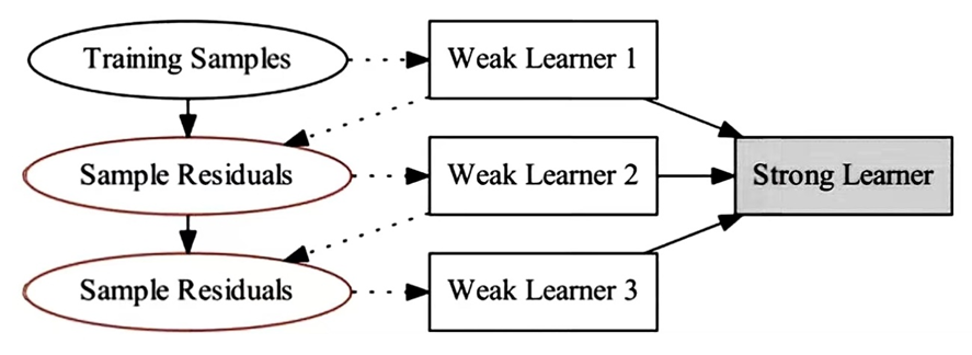
Figure 1: GBR model structure diagram.

As we can see from Figure 1, GBR gradually improves the predictive power of the model by iteratively adding weak learners (usually decision trees). The execution process is roughly divided into the following steps:

Step 1: Initialize the model The GBR algorithm starts with an initial model, which is usually the mean of the target values:

\( {f_{0}}(x)=argminc\sum _{i-1}^{n} L({y_{i}},c)\ \ \ （1） \)

Where \( L \) is the loss function, y_i is the true value of the \( i \) th observation, and c is a constant.

Step 2: Iterative training, in each iteration, the GBR algorithm performs the following steps:

1. Calculate the residual: The residual is the difference between the predicted value of the current model and the actual value:

\( {r_{mi}}=-[\frac{∂L({y_{i}},{f_{m}}-1({x_{i}}))}{∂{f_{m}}-1({x_{i}})}]\ \ \ (2) \)

Where, \( {r_{mi}} \) is the residual of the \( i \) th observation in the \( m \) th iteration.

2. Train the tree: Train a new decision tree \( {h_{m}}(x) \) with the residual \( {r_{mi}} \) as the target value.

Step 3: Update the model: Add the newly trained decision tree to the model and use the learning rate η to control its contribution, resulting in the model after the m th iteration:

\( {f_{m}}(x)={f_{m}}-1(x)+η{h_{m}}(x)\ \ \ （3） \)

2.2. Principle of Long Short-Term Memory (LSTM) algorithm

The Long Short-Term Memory Network (LSTM) is a specialized variant of Recurrent Neural Networks (RNN) explicitly designed to address the challenges of gradient vanishing and gradient explosion that traditional RNNs encounter when handling long-term dependencies. By incorporating a series of gating mechanisms to regulate the flow of information, LSTM excels in modeling time series data, particularly when capturing long-term dependencies within such datasets.

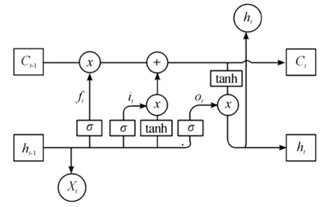
Figure 2: LSTM model structure diagram.

The core architecture of LSTM is characterized by three principal components: the Forget Gate, Input Gate, and Output Gate, along with a memory mechanism known as the Cell State.

Cell State: This is a path through the entire LSTM network that allows information to pass on undisturbed. The memory cell lies at the heart of the LSTM architecture, enabling it to retain and transmit information over extended periods.

Forget Gate: The forget gate governs the information to be discarded from the memory cell. By processing the current input and the previous hidden state, it generates a value between 0 and 1 through a Sigmoid function, thereby regulating the extent to which the memory is forgotten. The formula for the forget gate is as follows:

\( {f_{t}}=σ({W_{f}}\cdot [{h_{t-1}},{x_{t}}]+{b_{f}})\ \ \ （4） \)

Where \( {f_{t}} \) is the output of the forget gate, \( σ \) is the Sigmoid activation function, \( {W_{f}} \) is the weight matrix, \( {h_{t-1}} \) is the hidden state at the last time, \( {x_{t}} \) is the current input, and \( {b_{f}} \) is the bias term.

Input Gate: The input gate governs the incorporation of new information into the memory cell. Utilizing a Sigmoid function, it produces a value that regulates the updating process. Simultaneously, a tanh function generates candidate values for the memory cell, which are added to the memory cell under the control of the input gate. The input gate is formulated as follows:

\( {i_{t}}=σ({W_{i}}\cdot [{h_{t-1}},{x_{t}}]+{b_{i}})\ \ \ (4) \)

\( {\widetilde{C}_{t}}=tanh{({W_{c}}\cdot [{h_{t-1}},{x_{t}}]+{b_{c}})}\ \ \ (5) \)

Where \( {i_{t}} \) is the output of the input gate and \( {\widetilde{C}_{t}} \) is the new candidate memory cell value.

Output Gate: The output gate governs the hidden state, or the network's output, at the current time step. It utilizes a Sigmoid function to regulate the output from the memory unit, which is then combined with the memory unit's results, processed through the tanh function, to produce the final hidden state. The output gate is formulated as follows:

\( {o_{t}}=σ({W_{o}}\cdot [{h_{t-1}},{x_{t}}]+{b_{o}})\ \ \ (7) \)

\( {h_{t}}={o_{t}}\cdot tanh{({C_{t}})}\ \ \ (8) \)

Where \( {o_{t}} \) is the output of the output gate, \( {h_{t}} \) is the current hidden state, and \( {C_{t}} \) is the updated memory cell state.

LSTM (Long Short-Term Memory) networks dynamically regulate the flow of information through three gate mechanisms. The forget gate determines which information should be discarded from the memory cell, while the input gate decides which new data should be stored. Additionally, the output gate controls what information is released at each time step, taking into account not only the current input but also the long-term information retained in the memory cell.

This architecture allows LSTMs to effectively capture long-range dependencies without encountering the vanishing or exploding gradient issues that can arise in traditional RNNs when processing long time steps.

2.3. Principle of double-layer Long Short-Term Memory Network (D-LSTM) algorithm

The Double-layer Long Short-Term Memory network (D-LSTM) builds upon the single-layer LSTM, enhancing its capacity to model complex time series data by increasing the network's depth. Unlike the single-layer LSTM, the D-LSTM consists of two levels of LSTM units, with the output of the first layer serving as the input to the second, thereby creating a more intricate pathway for information flow.

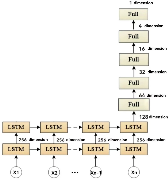
Figure 3: Schematic diagram of the two-layer LSTM network structure.

In D-LSTM, the input data is initially processed by the first layer of LSTM units, which are responsible for extracting temporal features from the input sequence. Unlike traditional shallow networks, D-LSTM uses the output from the first layer as the input to the second layer, allowing the model to perform multi-level feature abstraction. The second LSTM layer further refines the data based on the features extracted by the first layer, capturing more complex, higher-level temporal patterns. This layered approach to feature extraction enhances the representational power of D-LSTM, enabling it to model long-term dependencies while preserving its ability to capture local temporal features.

The continuous flow of information between layers allows D-LSTM to effectively handle both short-term and long-term dependencies at varying levels, thereby improving the model's performance in addressing complex temporal tasks.

3. Data acquisition and preprocessing

3.1. Data acquisition

The stock data used in this article is obtained by calling the TuShare API interface. TuShare is a Python-based data interface library that provides various data of Chinese financial markets, including stocks, futures, funds, and so on.

Take the data of Yangtze Power (6009000.SH) as an example, the data acquired through TuShare, and the time range is from November 18, 2003 to August 31, 2024. The dataset contains 55 impact factors, of which 8 columns have missing values.

3.2. Data preprocessing

(1) Data authenticity test: Compare several samples randomly selected from the original data with the data on the Oriental Fortune website to confirm that the data are completely consistent.

(2) Outlier handling: For missing values, we delete the row directly because they account for less than 1% of the total. Data mean replacement is used for excessively large and small outliers.

(3) Feature engineering: After many simulation experiments, finally screening out the 'open price before the right ',' high price before the right ',' low price before the right ',' yesterday closed price before the right ','CCI','MACD',' volume' and other features as the model input features, effectively improving the model performance.

(4) Normalization: Min-max normalization is applied to rescale the data within a specified range, thereby ensuring a more uniform distribution of the values.

(5) Data split: The dataset is partitioned into two subsets: 80% for the training set and 20% for the test set. The training set is utilized to train the model, while the test set is reserved for assessing the model's performance.

4. Model building

4.1. Gradient boosted regression with machine learning

Gradient Boosting Regression (GBR) is an ensemble learning technique that integrates multiple weak learners to enhance the model's predictive performance. This approach allows the GBR model to better capture the complex nonlinear relationships within the data, resulting in high accuracy and robustness, particularly in financial time series forecasting.

To further improve the prediction performance of the GBR model, we employ Randomized Search Cross-Validation to optimize its hyperparameters. This method works by randomly sampling within a specified parameter space to identify the optimal combination of parameters, with cross-validation applied after each sampling to ensure the model’s reliability.

In the random search process, we randomly sampled the parameter space 10 times and employed 3-fold cross-validation to assess the performance of each parameter set. To expedite model training, we leveraged parallel processing. Ultimately, the random search identified the optimal parameter combination, and the GBR model was trained using this configuration.

As the GBR model requires input data in a two-dimensional format, we first transformed the training and test sets from a three-dimensional structure (samples, time steps, features) into a two-dimensional structure (samples, expanded features) to meet the input requirements of GBR. To ensure the interpretability of the prediction results, we reversed the normalization process, restoring both the predicted and actual values to the original data scale.

Next, we calculated the residual prediction errors for both the training and test sets, saving these residuals as csv files. These residuals were then used to compute the Akaike Information Criterion (AIC) and Bayesian Information Criterion (BIC), providing a foundation for the subsequent quantitative analysis of the models' goodness of fit.

4.2. Construction of Long Short-Term Memory Network Model (LSTM)

In addition to the GBR model, in this study, we also construct a single-layer long Short-Term Memory (LSTM) network and a two-layer LSTM network model to predict stock price movements. LSTM, a type of Recurrent Neural Network (RNN), is adept at capturing long-term dependencies in time series data, making it particularly well-suited for processing financial data with temporal dependencies.

In the S-LSTM model, the network begins with an LSTM layer containing 64 units, where the input data consists of both time steps and features. This LSTM layer is followed by several fully connected layers, ultimately producing a single output node for prediction. The total number of parameters in the model is 64,109, with 21,369 of those being trainable. Notably, the model contains no non-trainable parameters, allowing all parameters to be adjusted during training. Additionally, the parameters of optimizer are set to 42,740, and the model weights are updated through the optimization process.

In contrast to the single-layer LSTM, the double-layer LSTM (D-LSTM) increases the model’s complexity. The first LSTM layer comprises 256 units, and its output time series serves as input for the second LSTM layer, which contains 128 units. The design of the subsequent fully connected layers mirrors that of the S-LSTM. The total number of parameters in the D-LSTM model is 1,438,253, with 479,417 being trainable. Like the S-LSTM, the D-LSTM model has no non-trainable parameters, ensuring all parameters remain adjustable. Furthermore, the optimizer's parameter count is 958,836, enabling the D-LSTM model to continuously update its weights throughout the training process.

Both models output prediction results after training and testing, and the predicted values are adjusted by reverse normalization. In the prediction results of the model, we calculate the residuals on the training and test sets, and save the residuals as CSV files.

To further quantify the goodness-of-fit of the model, we calculated Akaike Information Criterion (AIC) and Bayesian Information Criterion (BIC) values based on the residuals.

5. Model application example

5.1. Example results

In this study, we take the stock data of Yangtze Power (6009000.SH) as an example, and use Gradient Boosting Regression (GBR), single-layer LSTM (S-LSTM), and double-layer LSTM (D-LSTM) to predict the price trend of this stock, respectively. Changjiang Power is an important listed company in China's power industry, and as one of the world's largest hydropower companies, its stock is widely followed. We train the model using historical data to forecast the company's stock price, and then use the residuals to calculate the AIC and BIC values.

In the visualization section, the output results from the test set are presented. The horizontal axis represents the time range of the test set, spanning 918 days, while the vertical axis reflects the projected closing price range, from 18 yuan per share to 32 yuan per share.

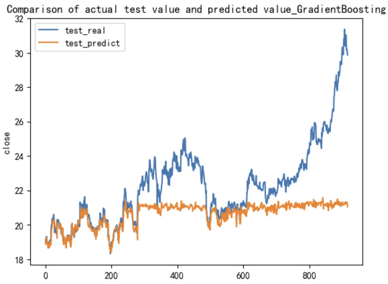
Figure 4: Visualization of the GBR model

Table 1: AIC and BIC values of the GBR model.

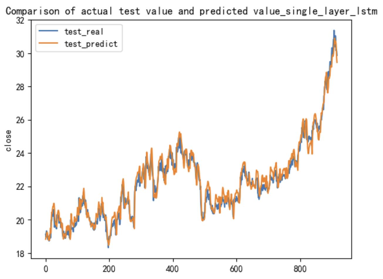
Figure 5: Visualization of the S-LSTM model

Table 2: AIC and BIC values of the S-LSTM model.

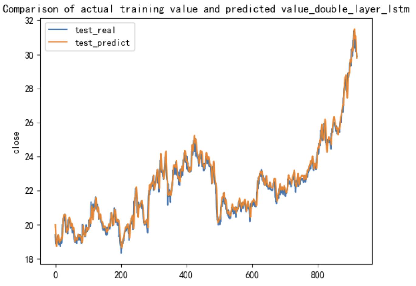
Figure 6: Visualization of the D-LSTM model

Table 3: AIC and BIC values of D-LSTM model.

5.2. Model Evaluation

5.2.1. Evaluation criteria

To comprehensively evaluate the performance of these models, we conducted a quantitative analysis of the goodness of fit and complexity of each model, mainly using Akaike Information Criterion (AIC) and Bayesian Information Criterion (BIC) as evaluation criteria.

1. Akaike Information Criterion (AIC)

The Akaike Information Criterion (AIC) is a metric that assesses a model's goodness of fit while accounting for its complexity. A lower AIC value indicates that the model better explains the variation in the data, without excessively increasing its complexity.[10]. The formula is as follows:

\( AIC=2k-2ln(L)\ \ \ (9) \)

Where k is the number of parameters of the model and L is the value of the log-likelihood function of the model.

2. Bayesian Information Criterion (BIC)

The Bayesian Information Criterion (BIC) is similar to the Akaike Information Criterion (AIC), but it incorporates a more stringent penalty term to discourage unnecessary increases in model complexity. As a result, BIC imposes a harsher penalty on models with a large number of parameters.[9] The formula for BIC is as follows:

\( BIC=ln{(n)}k-2ln{(L)}\ \ \ (10) \)

Where n is the number of samples, k is the number of parameters of the model, and L is the log-likelihood value.

5.2.2. Evaluation Conclusions

Table 4: Model evaluation data sheet(600900.SH).

Table 5: Model evaluation data sheet(000933.SZ).

Table 6: Model evaluation data sheet(000001.SZ).

In terms of the AIC values, it is evident that the double-layer LSTM model exhibits the lowest AIC, signifying the optimal fit to the data. This value represents the minimum in the dataset, thereby demonstrating the model's superior performance in capturing the underlying patterns. The single-layer LSTM follows, with a slightly higher AIC, while the gradient boosting regression (GBR) model shows a relatively higher AIC. These findings indicate that the double-layer LSTM model provides a more effective explanation of the data compared to both the single-layer LSTM and GBR models, independent of any considerations regarding overfitting.

The calculated BIC values are consistent with the trend of AIC values, and the double-layer LSTM model has the smallest BIC value, indicating that it achieves an optimal balance between goodness of fit and model complexity. The BIC value of the single-layer LSTM model is the second, indicating that it still maintains a good fitting effect while reducing the complexity. In contrast, the Gradient Boosted Regression (GBR) model has the largest BIC value, indicating that it is not as good as the LSTM model in this stock price prediction task. Although the number of parameters of the GBR model is relatively small, its lower complexity does not significantly improve the performance of the model.

6. Conclusion

This paper constructs and compares the application performance of Gradient Boosting Regression (GBR), single-layer LSTM and double-layer LSTM models in the stock price prediction of Yangtze River Power (600900.SH). The results of the experiment indicate that the double-layer LSTM model performs best in both evaluation indicators AIC and BIC, and the prediction accuracy of the stock price has reached a higher level, which is suitable for application in scenarios with high accuracy requirements. The single-layer LSTM model strikes a balance between prediction accuracy and model efficiency, all while maintaining low complexity. This makes it well-suited for practical applications that face constraints in computing resources. In contrast, the GBR model fails to adequately capture the long-term dependencies within the time series, leading to higher AIC and BIC values. As a result, its performance in this prediction task is inferior to that of the LSTM model.

There are still several problems and deficiencies in this study: first, the use of the closing price as the output of the prediction results in this study easily makes the results affected by the historical price trend, which may lead to the model being too dependent on the price trend in the long run, while ignoring the characteristics of short-term market fluctuations. In the subsequent research, the data such as return value or return rate can be selected as the output results to filter out the influence of absolute price trend on the model prediction, which is more effective in capturing the market's volatility. Secondly, the parameter setting of the GBR model has some limitations. Although grid search can optimize the performance of the model to a certain extent, there is no relevant theory that clearly proposes the optimal interval or configuration of each parameter. Therefore, the parameter selection of GBR mainly depends on the experiment and tuning process, which may lead to blindness in parameter selection and instability in model performance in practice. In addition, the dependence of LSTM model on long sequences still has limitations, which may lead to the loss of partial information. Future research could delve deeper into optimizing the model's computational complexity and enhancing its capacity to process long-sequence data, all while preserving its predictive accuracy.

References

[1]. Xiong, T., Bao, Y., & Hu, Z. (2014). Multiple-output support vector regression with a firefly algorithm for interval-valued stock price index forecasting. Knowledge-Based Systems, 55, 87-100.
[2]. Eling, M., Faust, R., & Others. (2010). The performance of hedge funds and mutual funds in emerging markets. CFA Digest, 40(3), 3-5.
[3]. Li, Q., Wang, T., & Gong, Q. (2014). Media-aware quantitative trading based on public Web information. Decision Support Systems, 61, 93-105.
[4]. Karim, F., Majumdar, S., Darabi, H., & Others. (2018). LSTM fully convolutional networks for time series classification. IEEE Access, 6(99), 1662-1669.
[5]. Al-Fattah, S. M. (2019). Artificial intelligence approach for modeling and forecasting oil-price volatility. SPE Reservoir Evaluation & Engineering, 22(3), 817-826.
[6]. LeCun, Y., Bengio, Y., & Hinton, G. E. (2015). Deep learning. Nature, 521(7553), 436-444.
[7]. Sang, C., & Pierro, M. D. (2019). Improving trading technical analysis with TensorFlow Long Short-Term Memory (LSTM) Neural Network. The Journal of Finance and Data Science, 5(1), 1-11.
[8]. Zhao, C. (2014). Application of dynamic neural network in quantitative investment forecasting. (Master's thesis, Fudan University, Shanghai).
[9]. Schwarz, G. E. (1978). Estimating the dimension of a model. Annals of Statistics, 6(2), 461-464. doi:10.1214/aos/1176344136.
[10]. Burnham, K. P., & Anderson, D. R. (2002). Model selection and multimodel inference: A practical-theoretic approach (2nd ed.). New York: Springer-Verlag. ISBN 0-387-95364-7.
Cite this article
Wang,R.;Wang,J.;Wang,H. (2025). Comparative Study on the Application of Gradient Boosting Regression and Single/Double-Layer LSTM Models. Advances in Economics, Management and Political Sciences,158,99-109.
Data availability
The datasets used and/or analyzed during the current study will be available from the authors upon reasonable request.
Disclaimer/Publisher's Note
The statements, opinions and data contained in all publications are solely those of the individual author(s) and contributor(s) and not of EWA Publishing and/or the editor(s). EWA Publishing and/or the editor(s) disclaim responsibility for any injury to people or property resulting from any ideas, methods, instructions or products referred to in the content.
About volume
Volume title: Proceedings of CONF-BPS 2025 Workshop: Sustainable Business and Policy Innovations
© 2024 by the author(s). Licensee EWA Publishing, Oxford, UK. This article is an open access article distributed under the terms and
conditions of the Creative Commons Attribution (CC BY) license. Authors who
publish this series agree to the following terms:
1. Authors retain copyright and grant the series right of first publication with the work simultaneously licensed under a Creative Commons
Attribution License that allows others to share the work with an acknowledgment of the work's authorship and initial publication in this
series.
2. Authors are able to enter into separate, additional contractual arrangements for the non-exclusive distribution of the series's published
version of the work (e.g., post it to an institutional repository or publish it in a book), with an acknowledgment of its initial
publication in this series.
3. Authors are permitted and encouraged to post their work online (e.g., in institutional repositories or on their website) prior to and
during the submission process, as it can lead to productive exchanges, as well as earlier and greater citation of published work (See
Open access policy for details).