1. Introduction

People are increasingly placing greater importance on their living standards. This is reflected not only in material life but also in the growing demand for spiritual, cultural, and environmental needs. With the intensification of urban expansion, more and more issues related to livability are emerging, such as traffic congestion caused by a large influx of population, rising housing prices, and environmental pollution due to industrial development, which makes ecological construction urgent. Today, people’s attention to urban livability goes beyond the economic and political development of cities. It also encompasses factors such as ecological environment, transportation convenience, social security, healthcare standards, cultural atmosphere, and the comfort of living conditions. This paper will analyze five aspects—economic development, social harmony, cultural education, ecological environment, and living comfort—by constructing a livable city model.

The livability index for constructing the livable city model is based on weight analysis of real data. The earliest domestic research on residential environment evaluation was proposed by Mr. Wu Liangyong in 1990. He developed a research method based on different needs from different populations, advocating an analysis of human living environments from four aspects: social environment, economic development, ecological environment, and cultural arts. Thus, he established the scientific theoretical system of the human living environment [1]. In China, the main focus of livable city evaluation has been on employment opportunities, the natural environment around daily life, and the cultural environment around daily life. At the same time, it is essential to maintain the sustainable development of cities in both ecological culture and economic construction. The current livable city evaluation models in China are relatively simple, with most analysis conclusions based on a single objective or subjective method. A scientifically representative mainstream livable city analysis has yet to be established. Some experts believe that a livable city should be one that offers convenient living, with advanced transportation, abundant educational resources, and cutting-edge medical technology; while others argue that a livable city is one with abundant natural resources, a pleasant climate, and is free from industrial development, thus supporting human ecological reproduction.

In 1973, a group of experts led by Johnston proposed that the livable environment for human habitation consists of three major factors: environmental factors outside of humans, environmental factors between individuals, and the geographic location of the residential area [1]. Due to the excessive exploitation of natural resources and the increasing expansion of industrial construction, the deterioration of the natural environment has attracted widespread attention. Consequently, in 1996, the United Nations put forward two key concerns: “adequate housing for all” and “sustainable development of human settlements in the urbanization process” [1]. In the 2017 report of Monocle magazine, it was stated that based on factors such as city safety, urban development, and public transportation, Tokyo, Japan, ranked first, and Hong Kong, China, entered the rankings [2]. The authoritative foreign media The Economist pointed out that the four aspects influencing the ranking of livable cities are: resource abundance, widespread services, personal safety, and sound infrastructure. Based on these four aspects, nine smaller factors are identified to determine the livability score of a city [3]. Currently, research on how to analyze whether a city is livable has become a global focus.

2. Overview of Livable Cities

2.1. Analysis of the Connotation of Livable Cities

A livable city is generally considered to be a city with a beautiful natural environment, pleasant climate, and conducive to human health. However, from the perspective of urban development and planning, a livable city not only involves ecological civilization construction but should also include economic development and the construction of public facilities. In terms of the standards used to assess cities, the livability score of a city is primarily based on various factors that determine the livability of a city. For most people, the selection of a livable city is subjective and lacks scientific basis. Different groups have varying understandings of a city’s livability. Young and middle-aged people tend to judge a city’s livability based on social resources such as employment opportunities, convenience, and healthcare conditions, while elderly people hope that a city not only protects the natural environment but also develops infrastructure and economic construction while meeting residents’ demands for a healthy living environment [4]. The most common requirements for whether a city is livable include: the safety of city travel, the completeness of public health construction, the convenience of travel, and the ecological suitability of the living environment. Higher-level housing demands include whether the city has a rich cultural atmosphere, abundant educational resources, and whether personal development opportunities can meet the needs of both new and past graduates in the city.

2.2. Related Factors of Livable Cities

The selection of livable city model indicators is based on different needs, with the key factor being whether the city meets the criteria for economic livability. At the same time, the surrounding natural environment of the city is also a focus of concern for residents. When analyzing the objective environmental conditions that constitute a livable city, residents’ subjective intentions can cause fluctuations in the importance of livability indicators. Only by integrating subjective thoughts and objective elements through mathematical models can an accurate livability analysis model be constructed.

2.3. Construction of Livable City Model

This paper divides the determining factors of a livable city into six components: economic development, social harmony, cultural and educational resources, transportation convenience, ecological environment quality, and public safety [5]. The selection of indicators follows three principles:

2.3.1. Holistic Nature

A city is composed of multiple aspects, determined by various factors, each with different impacts. Some factors may influence others, so the overall nature of the indicators needs to be considered.

2.3.2. Representativeness

The number of indicators selected to construct the livable city model is limited. If there are too many factors, some may be redundant, with information from one factor covering that of another. Therefore, representativeness should be considered.

2.3.3. Operability

The selected indicators should be quantifiable and easy to operate, enabling a reflection of the livability of different cities [6].

This paper will consider all of these factors in constructing a comprehensive evaluation model for livable cities.

The data for this study primarily comes from the statistical yearbooks published by the Sichuan Provincial Bureau of Statistics. The data is divided into five major categories and 23 indicators: economic development, social harmony, cultural education, ecological environment, and living comfort. Among these, 12 indicators—such as GDP per capita, per capita disposable income of urban residents, average wage of employees, unemployment rate, coverage rate of basic pension insurance, coverage rate of basic medical insurance, coverage rate of unemployment insurance, green coverage rate in built-up areas, household waste treatment rate, sewage treatment rate, population density, and per capita housing area—are directly extracted from the statistical yearbook. The remaining ten indicators are calculated based on data from high school teacher-student numbers, university teacher-student numbers, number of students in high school education, resident population, number of high schools, public library holdings, cultural station collections, private car ownership, number of hospital beds, number of healthcare staff, and number of healthcare institutions, among other indicators. This analysis allows for comparisons of the same indicators across different prefecture-level cities with varying scales.

Table 1: Livable City Model Evaluation Indicators

3. Determination of Model Indicator Weights

3.1. Dimensionless Processing of Data

The differences in measurement units of various indicators can lead to disparities between the indicators, which in turn affects the accuracy of comparisons and influences the subsequent assignment of indicator weights. If arithmetic operations such as addition, subtraction, multiplication, or division are forced, excessively large or small values of certain indicators can result in inaccurate models. Therefore, it is necessary to eliminate the dimensionality of all indicator data. In this paper, range standardization is used for dimensionless processing [7], with the formula as follows:

\( {y_{ij}}=\frac{{x_{ij}}-min{({x_{i}})}}{max{({x_{i}})}-min{({x_{i}})}} \)

Where, y_ij is the dimensionless data, max(x_i) is the maximum value of the indicator, and min(x_i) is the minimum value of the indicator.

By using range standardization, the data is constrained between [0,1] for centralized analysis without changing the degree of dispersion between the data.

After normalization and range standardization, all indicators are positive, and the unit and inherent variable effects of different indicators are eliminated. This enables the subsequent calculation using methods such as the entropy weight method, principal component analysis, and AHP.

3.2. Basic Principles of Entropy Weight Method for Determining Weights and Its Analytical Steps

The entropy weight method is an objective weighting method. Therefore, the first step in assigning weights to the indicators in this paper is to use the entropy weight method to assess the importance of the indicators. According to the definition of the entropy weight method, the greater the uncertainty of an indicator, the more information it contains, and the greater its weight [8]. This paper calculates the weight of an indicator by evaluating the data variability of the same indicator. That is, the greater the data variability of the indicator, the greater its influence on the city’s livability.

The steps for calculating weights using the entropy weight method are as follows:

Step 1: Calculate the Proportion of Standardized Data

\( {p_{ij}}=\frac{{x_{ij}}}{\sum _{j=1}^{n}{x_{ij}}} \)

Where, x_ij is the standardized data of the indicator, and p_ij is the data proportion.

This step calculates the ratio of the j-th city’s data of the i-th indicator to the total value of the i-th indicator. It is used to analyze the degree of separation of the i-th indicator’s values between different cities.

Step 2: Calculate the Information Entropy of Each Indicator

\( {E_{i}}=-[ln⁡(n)]{⁡^{-1}}\sum _{j=1}^{n}{p_{ij }}ln{p_{ij}} \)

Where, E_i is the information entropy of the indicator, j = 1,…,n, and n represents the number of cities.

By summing the data proportions of the same indicator, indicators with larger data proportion differences will result in smaller entropy values than indicators with smaller data proportion differences. This reflects the amount of information contained in an indicator and serves as the basis for subsequent weight analysis.

The larger the value of the information entropy E_i, the lower the uncertainty of the indicator x_i, and the smaller the amount of information it contains. That is, the indicator has less influence on the city’s livability.

Step 3: Calculate the Weights of Each Indicator

\( {W_{i}}=\frac{1-{E_{i}}}{\sum _{i=1}^{k}(1-{E_{i}})} \)

Wi as the Weight of the Indicator

By treating the disorder and orderliness of an indicator as a whole, the orderliness of the indicators is calculated individually. The most systematic indicator is assigned the highest weight, followed by the assignment of weights to the remaining indicators. This approach effectively summarizes the characteristics of the indicators and provides a weight comparison based on the differences in the data, making it an objective and meaningful weight assignment method.

Through this process, the weight of each indicator’s influence on urban livability can be determined.

3.3. Determining Weights Using Principal Component Analysis (PCA)

The Principal Component Analysis (PCA) method identifies the principal components for five livability aspects and uses eigenvalues, indicator coefficients, and standardized principal component matrices to calculate the weight of each indicator. PCA is a method that eliminates redundant information by identifying correlations between indicators. For instance, if indicators A and B exhibit similar trends, their information is considered overlapping. PCA removes similar indicators and constructs new, uncorrelated indicators that retain all the information conveyed by the original indicators.

The steps for calculating weights using PCA are as follows:

Step 1: Treat Secondary Indicators as Factors Under Each Primary Indicator

Use statistical software, such as SPSS, for factor analysis to obtain the principal components under each primary indicator [9], including the component matrix, eigenvalues of the principal components, and principal component variance.

Step 2: Calculate Coefficients of Secondary Indicators in the Linear Combination of Each Principal Component [9]

\( {F_{iz}}=\sum _{j=1}^{n}{a_{ij}}{x_{ij}} \)

i = 1,2,3,4,5 (Primary Indicators)

z = 1,2 (Principal Components of Primary Indicators)

j = 1,2,3,4,5,6 (Secondary Indicators under Primary Indicators)

Here, x_j represents the principal components. In this study, there are five primary indicators and 22 secondary indicators. Each primary indicator consists of several secondary indicators, where x_j represents the principal components of a primary indicator. Using SPSS, the number of principal components and the standardized values of the secondary indicators in the principal components can be analyzed for each primary indicator.

\( {a_{i}}=\frac{{y_{i}}}{\sqrt[]{r}} \)

i = 1,2,3,,,22 (Secondary Indicators under Primary Indicators)

Since the number of primary indicators and principal components varies, the analysis simplifies to consider only the secondary indicators under each primary indicator, where the values of r (eigenvalues of the principal components) also vary and are not fixed.

Here, F_iz refers to the principal component, a denotes the coefficient, y represents the standardized value of a specific indicator in the principal component matrix, and r is the eigenvalue of the principal component. Dividing the standardized value in the principal component matrix by the square root of the eigenvalue gives the proportion of each secondary indicator under different principal components, which is the eigenvector.

Step 3: Calculating Indicator Weights Using Principal Component Variance [10]

\( {W_{i}}=\frac{\sum _{i=1}^{n}{s_{i}}{a_{i}}}{\sum _{i=1}^{n}{s_{i}}} \)

Here, S represents the variance of the principal components, a refers to the coefficients of the principal components in the secondary indicators, and Wi denotes the weight.

By calculating the variance of the principal components, the weight of each secondary indicator under the corresponding primary indicator can be determined. Since the urban livability model is a unique perceptual model based on human experience, the importance of all primary indicators is treated equally [11]. In this study, there are five primary indicators, each assigned a weight of 0.2. The weight of each secondary indicator under a primary indicator is multiplied by 0.2 to derive the weight values for all 22 indicators. Using the Principal Component Analysis method, dimensionality reduction is employed to streamline the data while retaining as much information as possible, making the data easier to explore and analyze visually.

3.4. AHP Validation of the Weight Qualification in Principal Component Analysis

The relationships among various factors can be hierarchical or parallel, depending on the degree of correlation between the factors. Using the Analytic Hierarchy Process (AHP) integrates data for decision-making, highlights the interconnections between factors, incorporates the calculated weights for analysis, and evaluates whether the weights of the factors correspond to their respective levels of importance [12].

The process of validating the weights obtained through Principal Component Analysis (PCA) using AHP involves three steps:

Step 1: Establishing the Judgment Matrix

The judgment matrix is constructed based on the weights of each layer derived from PCA.

Economic Development: Using per capita regional GDP as a reference, the importance of urban residents’ per capita disposable income and average wage is assigned.

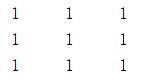
Figure 1: Economic Development Judgment Matrix

Social Harmony: Using the unemployment rate as a reference, the importance of the coverage rates of basic pension insurance, basic medical insurance, unemployment insurance, and the case-solving rate for public security incidents is assigned.

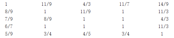
Figure 2: Social Harmony Judgment Matrix

Cultural and Educational Development: Using the ratio of teachers in high schools as a reference, the importance of the teacher ratio in regular higher education institutions, the number of enrolled high school students, the number of high schools, and the public library book collections per 100 people is assigned.

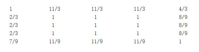
Figure 3: Cultural and Educational Development Judgment Matrix

Ecological Environment: Using the green coverage ratio of built-up areas as a reference, the importance of the rates of solid waste treatment and sewage treatment is assigned.

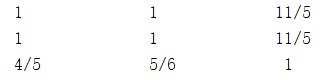
Figure 4: Ecological Environment Judgment Matrix

Living Comfort: Using population density as a reference, the importance of per capita housing area, per capita ownership of private vehicles, the number of hospital beds, the number of healthcare personnel, and the number of healthcare institutions is assigned.

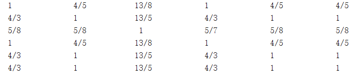
Figure 5: Living Comfort Judgment Matrix

Step 2: Performing Hierarchical Single Sorting and Consistency Check [13]

\( CI= \frac{t-n}{n-1} \)

Here, CI is the consistency index, t is the largest eigenvalue of the matrix, and n is the order of the matrix.

Table 2: Random Consistency Index (RI) Values

\( CR= \frac{CI}{RI} \)

Here, CR is the consistency ratio. If CR<0.1, the matrix is considered to have passed the consistency check, and its normalized eigenvector can be used as the weight.

Step 3: Performing Hierarchical Total Sorting and Consistency Check

\( CR= \frac{\sum _{i=1}^{M}{w_{i}}{CI_{i}}}{\sum _{i=1}^{m}{w_{i}}{RI_{i}}} \)

Here, CR is the consistency ratio, w represents the weight, CI is the consistency index, and RI is the random consistency index.

If CR<0.1, the hierarchical total sorting is considered to have passed the consistency check.

The purpose of employing the AHP method for weight analysis is to evaluate the consistency of the relative importance of each indicator. To achieve this, relative scales and matrix analysis are adopted, aiming to minimize difficulties in comparing indicators of different natures. This approach avoids confusion in determining the importance of indicators.

4. Research Steps and Results

The weights derived from the entropy weight method, principal component analysis, and validated using the Analytic Hierarchy Process were used as the initial data. The final weights were obtained through the following three steps [14]:

Weights from the Entropy Weight Method:

U = {u₁,u₂,…,u_n}

Weights from Principal Component Analysis:

Primary Indicator Weights: A = {a₁,a₂,a₃,a₄,a₅}

Secondary Indicator Weights: B = {b₁,b₂,…,b_n}

Step 1: Simple Integration of Secondary Weights Derived from AHP and PCA

The combined weights are represented as: T = {t₁,t₂,…,tn}

\( {t_{i}}=\frac{{u_{i}}{b_{i}}}{\sum _{i=1}^{n}{u_{i}}{b_{i}}} \)

i = 1,2,…,n

This step multiplies the weights obtained from the two methods to mitigate the overemphasis or underemphasis on any specific factor.

Step 2: Reallocation of Secondary Indicator Weights Based on Primary Indicators

The integrated weights are expressed as:

T = {t₁₁,t₁₂,t₁₃,t₂₁,t₂₂,t₂₃,t₂₄,t₂₅,t₃₁,t₃₂,t₃₃,t₃₄,t₃₅,t₄₁,t₄₂,t₄₃,t₅₁,…,t₅₆}

The normalized weights for each indicator are represented as:

D = {d₁₁,d₁₂,d₁₃,d₂₁,d₂₂,d₂₃,d₂₄,d₂₅,d₃₁,d₃₂,d₃₃,d₃₄,d₃₅,d₄₁,d₄₂,d₄₃,d₅₁,…,d₅₆}

\( {d_{ij}}= \frac{{t_{ij}}}{\sum _{j=1}^{k}{t_{ij}}} \)

i = 1,2,3,4,5; k = 3,5,5,3,6

Each indicator is grouped under its corresponding primary indicator, and weights are assigned within each group. This eliminates the influence of differing primary indicators on the 22 secondary indicators.

Step 3: Calculation of Final Weights

The secondary indicator weights B are multiplied by the normalized weights D to yield the final weights:

{w₁₁,w₁₂,w₁₃,w₂₁,w₂₂,w₂₃,w₂₄,w₂₅,w₃₁,w₃₂,w₃₃,w₃₄,w₃₅,w₄₁,w₄₂,w₄₃,w₅₁,…,w₅₆}

\( {w_{ij}}= {b_{i}}* {d_{ij}} \)

In this study, it is assumed that the importance of all primary indicators is equal, so b_i is set at a fixed value of 0.2. The importance values of the primary indicators are distributed to their corresponding secondary indicators to produce the final weights that integrate the results of the two methods. The entropy weight method emphasizes the information quantity and the degree of data variation among indicators. However, this method may overemphasize indicators with high information content or large variations, leading to potential distortions when data volume is limited. Conversely, PCA assigns weights based on dimensionality reduction, simplifying data interpretation and analysis.

By combining the weights using a multiplicative approach, this study reduces the bias caused by the high data information in the entropy method while addressing the potential inaccuracies in PCA’s weight estimations. The resulting weights more objectively reflect the relative importance of indicators affecting urban livability.

The final weight values for the indicators are shown in Table 3.

Table 3: Indicator Weights

5. Conclusion

Based on the analysis of livable city indicator weights derived from the statistical yearbook data of Sichuan Province, the importance of the five aspects—economic development, social harmony, culture and education, ecological environment, and living comfort—is relatively balanced. Among these, the secondary indicator “green coverage rate” under the ecological environment holds the highest weight. This indicates that the critical evaluation standard for a livable city lies in residential environmental greening, aligning with the United Nations’ advocacy for low-carbon and environmentally friendly initiatives. Therefore, I plan to incorporate additional environmental indicators, such as greenhouse gas emissions, in future research to enhance the livable city model.

References

[1]. Shao, S. (2012). A review of domestic and international research on livable city theory [J]. Modernization of Shopping Malls, (01), 97–99.
[2]. Jiang, Y. H., Zhen, F., & Wei, Z. C. (2009). The practice of building livable cities abroad and its implications [J]. International Urban Planning, 24(04), 99–104.
[3]. Development of a liveable city index (LCI) using multi-criteria geospatial modelling for medium-class cities in developing countries. (2018). Sustainability, 10, 520.
[4]. Zhang, W. Z. (2007). Discussion on the connotation and evaluation index system of livable cities [J]. Urban Planning Journal, (03), 30–34.
[5]. Li, L. P., & Wu, X. Y. (2007). Research on the evaluation index system of livable cities [J]. Journal of the Party School of the CPC Jinan Municipal Committee, (01), 16–21.
[6]. Hu, F. X., & Hu, X. J. (2014). Construction of an evaluation index system for urban livability [J]. Ecological Economy, 30(08), 42–44.
[7]. Wang, H., & Guo, C. Y. (2017). Research on the impact of linear dimensionless methods on the index weight of entropy methods [J]. China Population, Resources, and Environment, 27(S2), 95–98.
[8]. Yang, X. Q., Wang, Q., Wang, R. F., & Wang, L. (2017). Analysis of urban livability based on the entropy weight method [J]. Science and Technology Economic Guide, (35), 85–86.
[9]. Wei, Q. J., & Tian, J. X. (2018). Evaluation model of urban livability based on principal component analysis [J]. Residence, (03), 191.
[10]. Jiang, Y., Zhu, J. M., Wang, Y., & Liang, J. (2018). Research on livable city evaluation indicators based on principal component analysis [J]. Journal of Jiaozuo University, 32(01), 85–89.
[11]. Yan, H. Q., Niu, W. H., & Han, H. L. (2017). Objective weighting method for constructing index weights based on principal component analysis [J]. Journal of Jinan University (Natural Science Edition), 31(06), 519–523.
[12]. Wang, R. S., Zhou, F., & Chen, G. (2018). Fuzzy evaluation model of livable cities based on analytic hierarchy process [J]. China High-Tech Zones, (02), 6.
[13]. Li, Y. X., Zhu, J. M., Li, P. P., & Wu, M. H. (2017). Livable city evaluation model based on AHP and factor analysis [J]. Journal of Teachers’ Science, 37(08), 15–19.
[14]. Chen, Y. L. (2017). Application of improved analytic hierarchy process and entropy weight method fusion technology—Based on the innovation-driven development evaluation model. Frontiers of Social Sciences, 6(6), 728–734.
Cite this article
Hu,H. (2025). A Livable City Model Based on the Integration of AHP and Entropy Weight Method. Advances in Economics, Management and Political Sciences,164,7-17.
Data availability
The datasets used and/or analyzed during the current study will be available from the authors upon reasonable request.
Disclaimer/Publisher's Note
The statements, opinions and data contained in all publications are solely those of the individual author(s) and contributor(s) and not of EWA Publishing and/or the editor(s). EWA Publishing and/or the editor(s) disclaim responsibility for any injury to people or property resulting from any ideas, methods, instructions or products referred to in the content.
About volume
Volume title: Proceedings of the 4th International Conference on Business and Policy Studies
© 2024 by the author(s). Licensee EWA Publishing, Oxford, UK. This article is an open access article distributed under the terms and
conditions of the Creative Commons Attribution (CC BY) license. Authors who
publish this series agree to the following terms:
1. Authors retain copyright and grant the series right of first publication with the work simultaneously licensed under a Creative Commons
Attribution License that allows others to share the work with an acknowledgment of the work's authorship and initial publication in this
series.
2. Authors are able to enter into separate, additional contractual arrangements for the non-exclusive distribution of the series's published
version of the work (e.g., post it to an institutional repository or publish it in a book), with an acknowledgment of its initial
publication in this series.
3. Authors are permitted and encouraged to post their work online (e.g., in institutional repositories or on their website) prior to and
during the submission process, as it can lead to productive exchanges, as well as earlier and greater citation of published work (See
Open access policy for details).