1. Introduction

Momentum and reversal effects are two well-documented phenomena in the field of financial asset pricing. In recent years, research on momentum and reversal effects has primarily focused on theoretical models. Kelly, Moskowitz, and Pruitt use a conditional factor pricing model and instrumented principal components analysis (IPCA) to show that stock momentum and long-term reversal are predictive of future returns due to their correlation with time-varying risk exposures[1]. Nonetheless, these studies have predominantly been theoretical and have not comprehensively examined particular markets, especially the technology industry. Recent studies have begun to address this issue, with some concentrating on momentum and reversal effects within particular sub-sectors of the technology industry. For example, Huang, Shih, and Ke examine the semiconductor industry's technological evolution, use Lyapunov exponents to examine patent duration and find that the semiconductor industry's innovation has moved from an orderly to a chaotic phase[2]. Similarly, research on short-term momentum in financial markets, such as the S&P Composite stock price index, has found evidence supporting the profitability of trend-following strategies, though with challenges related to statistical test power[3]. However, there remains a lack of research that comprehensively examines momentum and reversal across different technology industries and compares the effects at the sector level and within individual firms. This paper first provides an overall insight into the momentum and reversal effects within the technology sector, followed by dynamic (time-series) and static (cross-sectional) analyses at the industry and company levels. Additionally, the Fama-MacBeth regression is employed to evaluate the robustness of these effects and control for risk factors[4-6]. This research contributes to the existing literature by offering a granular perspective on the momentum and reversal dynamics within the technology sector. The findings hold significance for both academia and practice, offering essential insights for portfolio managers, investors, and policymakers focused on sector-specific investment strategies and risk management within the technology sector.

2. Methodology

2.1. Variable Definitions and Calculation Methods

To explore the dynamic characteristics of momentum and reversal effects, this study introduces the concept of cumulative returns ( \( {R_{cumulative}} \) ) as the foundational measure of asset returns. Building on this, past returns ( \( {R_{past}} \) ) are further defined as the core variable for analysis and model construction, using data from Yahoo Finance for the period from January 2023 to December 2024[7]. Cumulative Returns reflects the total return performance of an asset over a designated timeframe. The formula for its calculation is as follows:

\( {R_{cumulative}}=\prod _{t=1}^{n}(1+{R_{t}})-1 \) (1)

Where \( {R_{t}}=\frac{{P_{t}}{-P_{t-1}}}{{P_{t-1}}} \) , and \( {P_{t}} \) represents the closing price of the asset at time t with n denoting the length of the cumulative period (e.g., monthly or quarterly).

This formula describes the total return over a specific time horizon. Past Returns serve as the core variable of this study, past returns are calculated using a rolling window approach based on the concept of cumulative returns. The formula is as follows:

\( {R_{past}}=\prod _{t=T-k}^{n}(1+{r_{i,t}})-1 \) (2)

Where T denotes the current time point, k represents the length of the time window (e.g. months or 6 months), and \( {r_{i,t}} \) is the monthly return of asset i at time t.

To further analyze the impact of different time windows on momentum and reversal effects, the study sets a rolling step size of 1 month to ensure sample dynamism and continuity.

2.2. Lost-Winning Portfolio Construction

To examine the presence of momentum effects and reversal effects, the sample stocks are grouped into winner and loser groups based on past returns performance. The top 30% (5 stocks) with the highest historical returns, as determined by Yahoo, are designated as the "winner group," whereas the bottom 30% (5 stocks) with the lowest historical returns are designated as the "loser group." [7][8] The remaining stocks in the middle are excluded from the analysis. This classification approach allows for a clear examination of momentum and reversal effects by focusing on the extremes of the return distribution.

Then the paper calculates the return of each group as the average return of the stocks within the group, calculated as follows:

\( {R_{group}}=\frac{1}{N}\sum _{i=1}^{N}{R_{i}} \) (3)

Where \( {R_{i}} \) represents the single-period return of stock i, and N is the number of stocks in the group.

Forthemore the paper calculate the momentum return and reversal return is defined as the difference in returns between the winner group and the loser group, with the formula as follows:

\( \begin{cases} \begin{array}{c} {R_{Momentum}}={R_{winners}}-{R_{losers}} \\ {R_{Reversal}}={R_{losers}}-{R_{winners}} \end{array} \end{cases} \) (4)

Where \( {R_{winners}} \) is the average return of the winner group, and \( {R_{losers}} \) is the average return of the loser group.

2.3. Regression Model Construction

To investigate the explanatory power of past industry returns or stock returns on future returns, the following cross-sectional regression model is used[9][10]:

\( {R_{future}}=α+β{R_{past}}+ϵ \) (5)

Where \( {R_{future}} \) represents the industry return or stock return over a future period (e.g., the next 3months or the next 6 months), and \( {R_{past}} \) represents the industry return over a past period (the last 3 months or the last 6 months). The sign and magnitude of the β coefficient reflect the significance and strength of the momentum or reversal effects.

If β is greater than 0, it indicates the presence of a momentum effect, whereas if β is less than 0, it suggests the presence of a reversal effect. To further compare the dynamic characteristics of different industries or stocks, the β coefficients from the regression model are calculated using a rolling window approach. At each time point, a fixed-duration time window (e.g., 3 months or 6 months) is retrospectively utilized to compute the β coefficient using historical data. The rolling window is thereafter pushed backward by one month at each interval, preserving the same window length. This approach captures the time-varying trends of the β coefficient, providing a clearer understanding of the dynamic nature of momentum and reversal effects[11][12].

The Fama-MacBeth two-step regression method is employed to evaluate the long-term predictive capacity of momentum factors on future returns. Initially, cross-sectional regressions are conducted at each time point to derive the time-series regression coefficients (β). In the second step, the mean of the regression coefficients across all time points is calculated to test its significance. The formula is as follows [4][5]:

\( \overline{β}=\frac{1}{T}\sum _{t=1}^{T}{β_{t}} \) (6)

The corresponding significance test is completed by calculating the following t-statistic:

\( t(\overline{β})=\frac{\overline{β}}{SE(\overline{β})} \) (7)

Where \( SE(\overline{β}) \) is the standard error of β.

3. Empirical Analysis

3.1. The Momentum Effect of the Overall Technology Sector

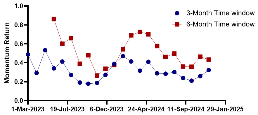
Figure 1: Monmentum return under different time-windows

3.1.1. Time Trend and Window Sensitivity Analysis

This paper calculates the return difference between winners and losers to represent the momentum effect and presents the image shown in Figure 1. It is observed that there is an overall downward trend in 2023, followed by a significant upward trend in early 2024. After reaching a peak, the returns exhibit a subsequent decline. The momentum return for the 6-month period surged swiftly in early 2023, attaining its zenith (about 0.8) mid-year before progressively diminishing, demonstrating increased overall volatility. Conversely, the 3-month period had comparatively minor swings, with returns predominantly ranging from 0.2 to 0.4. Overall, the return curve for the 6-month window demonstrated a significant growth trend in the early period, while the 3-month window was more stable. However, by the end of 2024, both trends converged, indicating a diminishing advantage of long-term returns.

3.1.2. Cross-Window Performance Comparison Analysis

In mid-2023 (June to September), returns from both windows converged due to consistent market volatility. However, in early 2024, the 6-month momentum return surged, driven by strong performance in sectors like technology. In mid-2023 (around July), the returns for the 6-month window were significantly higher than those for the 3-month window, demonstrating the 6-month window's stronger ability to capture medium- to long-term trends. By early 2024, the returns for both windows converged and briefly crossed, indicating that short-term and medium- to long-term market trends had become more aligned during this period. In the later half of 2024, despite the 6-month window yielding marginally superior returns, the volatility of both curves exhibited increasing similarity, indicating a gradual convergence in the efficacy of short- and long-term momentum strategies.

3.2. Comparison within Industries

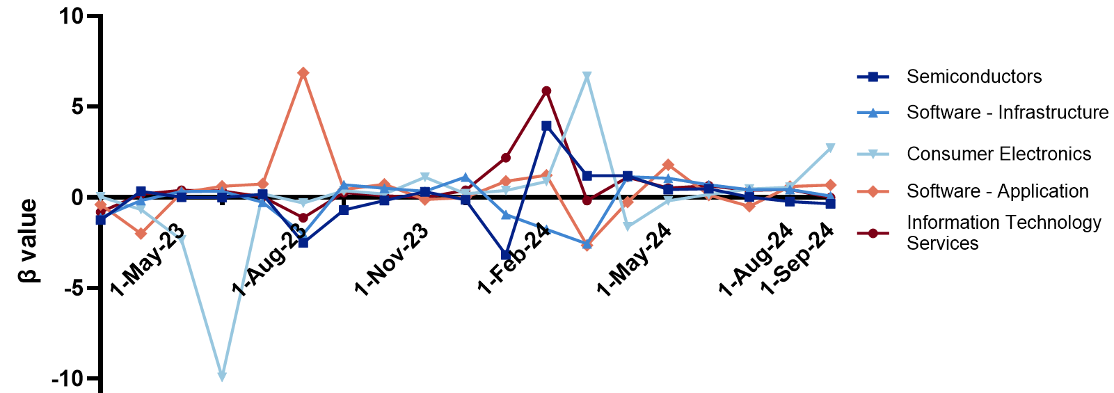
Figure 2: β value under the 3-month rolling window

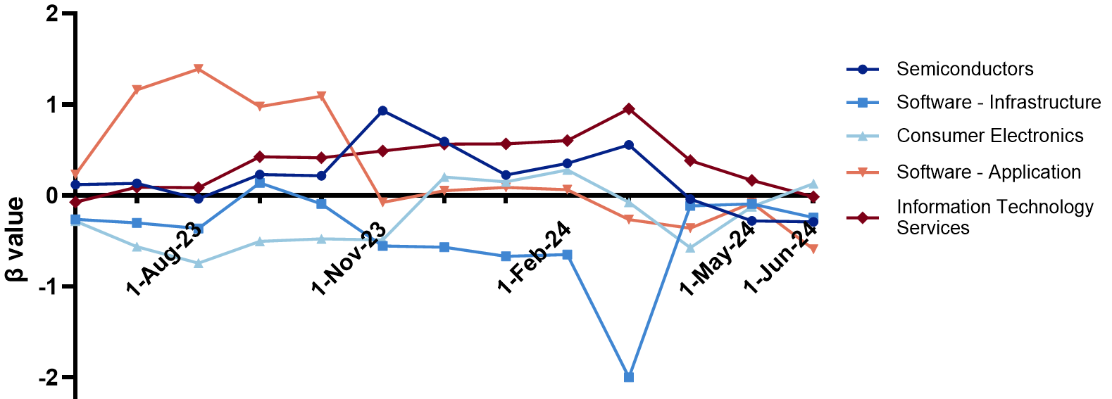
Figure 3: β value under the 6-month rolling window

3.2.1. Analysis of Time Series

The author calculates the β values using equation (5) and presents the results in Figure 2 and Figure 3. Comparing the 3-month and 6-month rolling windows highlights notable differences. While overall trends are consistent, the 6-month window produces smoother curves with fewer extremes, minimizing the impact of short-term volatility. In contrast, the 3-month window captures sharper fluctuations and more frequent reversals, reflecting stronger sensitivity to short-term market dynamics.

From the β value trends under 3-month and 6-month rolling windows, industries show distinct volatility and cyclicality patterns. The semiconductor industry exhibits stable trends, with β values near zero for most periods, likely due to the sector's technological maturity, which reduces volatility, and its market efficiency, which quickly incorporates new information. A significant positive peak is observed between December 2023 and January 2024, succeeded by a steep decrease, indicating overall weak momentum, potentially affected by transient market forces or external shocks. Conversely, the software-infrastructure sector exhibits greater volatility, with β values often oscillating between positive and negative. This instability is particularly pronounced in early 2024, showing a strong reversal effect. The consumer electronics industry displays extreme negative β values in May 2023 under the 3-month window, indicating a strong reversal effect. The 6-month window smooths these extremes, but volatility remains, reflecting inherent cyclicality and reversal tendencies. The software application industry shows mainly positive β values across both windows, with a peak from late 2023 to early 2024, reflecting a stable momentum effect. Lastly, the information technology services industry has consistent, predominantly positive β values, indicating persistent momentum, which is more evident under the 6-month window.

3.2.2. Cross Section Analysis

The Information Technology Services industry consistently leads, with positive beta values indicating strong momentum, while the Consumer Electronics industry lags, showing significant fluctuations and frequent negative values, reflecting a strong reversal effect.

Certain time points reveal anomalies in industry β values. In May 2023, the consumer electronics industry had extreme negative β values, possibly due to new product launches or shifts in consumer sentiment. In January 2024, the software and IT services industries exhibited significant positive β peaks, possibly due to increased tech investments or seasonal cycles. Additionally, the β values of consumer electronics and software applications showed notable differences between May 2023 and January 2024. The stable β values in the semiconductor and IT services sectors suggest these industries may be slow to react to market volatility. (Figure 2 and Figure 3)

3.3. Comparison within Stocks

3.3.1. Analysis of Time Series

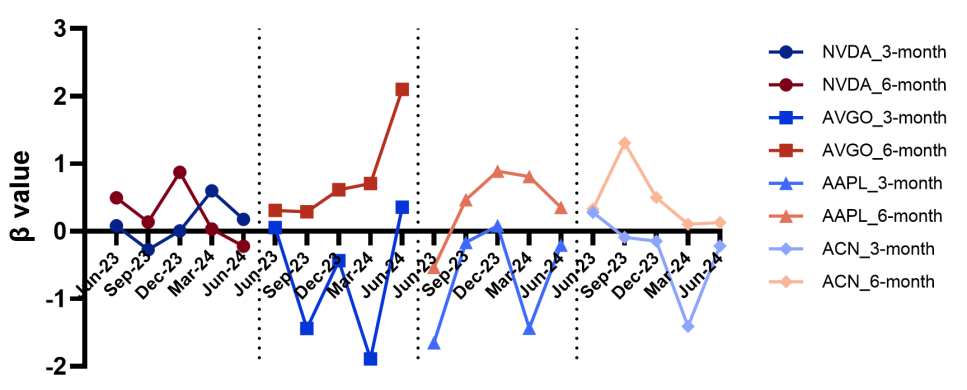
Figure 4: The β values of stocks with more pronounced momentum effects (partial)

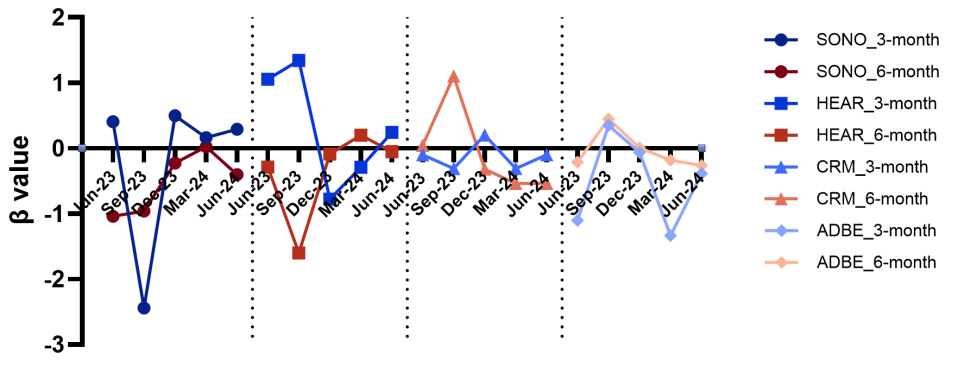
Figure 5: The β values of stocks with more pronounced reversal effects (partial)

The author selected a subset of stocks with notable β performance and categorized them based on different effects, presenting the results in Figure 4 and Figure 5. In the Semiconductor Industry, stocks like NVDA, AVGO exhibit significant momentum effects in a six-month window. Significantly, AVGO's β exceeded 2 at the onset of 2024, indicating heightened sensitivity to industry changes and substantial momentum impacts. Likewise, ACN (IT services sector) and AAPL (Consumer Electronics sector) exhibit persistent momentum effects, with their β maintaining positive throughout six-month intervals.

Conversely, reversal effects are more pronounced in the Consumer Electronics industry, particularly for SONO and HEAR, whose β values are mostly negative. HEAR, for instance, exhibited a sharp decline in beta after May 2023, followed by a quick recovery, likely driven by earnings reports or market sentiment shifts. Similarly, in the Software-Application industry, CRM(Software - Application industry)and ADBE (Software - Infrastructure industry) experienced a notable reversal in its β , dropping from positive to negative in late 2023 and early 2024.

It can be observed that there is significant time window dependence in the analysis. Momentum effects are particularly window-dependent. Stocks depicted in Figure 4 exhibit pronounced momentum during the six-month period, whereas the three-month period reveals significant volatility, underscoring the persistence of long-term trends and the emergence of short-term momentum. Figure 5 illustrates that reversal effects exhibit greater consistency over time intervals, although short-term volatility is more pronounced in extended periods.

3.3.2. Cross Section Analysis

In the semiconductor sector, AVGO's average β (0.6123) is significantly higher than NVDA (0.1378) and AMD (0.1586), indicating its strongest momentum effect in the long-term. In the Software - Infrastructure industry, Oracle (ORCL) exhibits the largest beta fluctuations, reflecting its higher sensitivity to market changes compared to Microsoft (MSFT) and Adobe (ADBE). The consumer electronics industry displays notable heterogeneity, with Sonos (SONO) and Turtle Beach (HEAR) having negative betas, while Apple's (AAPL) beta remains relatively high, reinforcing its position as a core stock. In the Information Technology Services sector, Accenture (ACN) displays greater momentum effect with higher average β (0.0366, 0.6153) than IBM and FI.

3.4. Significance Analysis (t-value)

Table 1: Comparison of key significance indicators

Table 1 presents the calculated average β and t-values for the companies and industries. In the semiconductor industry, AMD and AVGO show significant long-term momentum with t-values of 2.6984 and 4.5456 in the 6-month window, while NVDA's t-values are insignificant, indicating unreliable β estimates. The software-infrastructure sector often has diminished impacts; however, Oracle demonstrates a notable long-term reversal with a t-value of -4.0107, signifying susceptibility to market volatility, whilst Microsoft and Adobe have minor β values.

In consumer electronics, SONO and HEAR exhibit strong reversal effects with negative β values and notable t-values in both short- and long-term windows. Apple shows both long-term momentum (t = 2.7448) and short-term reversal (t = -2.2958), reflecting dual market roles. The stocks in the Software - Application industry generally show no significant momentum or reversal effects.

The IT services industry shows notable long-term momentum, led by Accenture (t = 4.1530) and IBM (t = 6.3896), though IBM shows short-term reversal tendencies (t = -3.0042). FIS has strong long-term momentum (t = 4.4098) but lacks short-term significance.

4. Conclusion

The momentum effect in the overall technology sector exhibits fluctuations over time, with notable peaks and troughs; the overall trend suggests moderate momentum returns. The information technology services and software-application industries exhibit stronger momentum effects, with consistently positive β values across most periods. This may arise from their dependence on enduring technical trends, consistent demand, and incremental adoption cycles. Conversely, the consumer electronics and software infrastructure sectors have significant reversal effects, marked by abrupt volatility and recurrent β value reversals. The semiconductors industry demonstrates relatively stable β values with limited momentum or reversal effects, reflecting its slower response to market cycles and its position as a foundational sector that often follows broader economic and technological trends. Overall, these differences underscore the heterogeneity among industries, driven by distinct structural and market dynamics. WIn the analysis of momentum and reversal effects among companies, it is observed that momentum effects are prevalent in large, innovative firms (e.g., AAPL, NVDA, ACN), whereas reversal effects frequently occur in smaller-cap companies (e.g., HEAR, CRM), generally coinciding with significant events or market corrections. This highlights the distinct market dynamics driven by industry and company size. The limitations of this paper lie in analyzing only a subset of leading companies and industries within the U.S. technology sector, with limited data coverage and without considering the impact of macroeconomic variables on momentum and reversal effects. Future research could expand to include more industries, regional markets, or integrate machine learning models to enhance predictive accuracy.

References

[1]. Kelly, B. T., Moskowitz, T. J., & Pruitt, S. (2021). Understanding momentum and reversal. Journal of financial economics, 140(3), 726-743.
[2]. Huang, H. C., Shih, H. Y., & Ke, T. H. (2024, August). Exporting the Innovative Momentum: The Case in the Semiconductor Industry. In 2024 Portland International Conference on Management of Engineering and Technology (PICMET) (pp. 1-9). IEEE.
[3]. Zakamulin, V., & Giner, J. (2022). Time series momentum in the US stock market: Empirical evidence and theoretical analysis. International Review of Financial Analysis, 82, 102173.
[4]. Fama, E. F., & MacBeth, J. D. (1973). Risk, return, and equilibrium: Empirical tests. Journal of Political Economy, 81(3), 607-636.
[5]. Fama, E. F., & French, K. R. (1996). Multifactor explanations of asset pricing anomalies. The Journal of Finance, 51(1), 55-84.
[6]. Jegadeesh, N., & Titman, S. (2001). Profitability of momentum strategies: An evaluation of alternative explanations. The Journal of Finance, 56(2), 699-720.
[7]. Yahoo Finance. (2023, January 1). Stock data for momentum and reversal effects analysis: January 2023 to December 2024. Yahoo Finance. https://finance.yahoo.com/
[8]. Vieri, M., Leon, F. M., Usman, B., & Mustafa, M. (2024) Analysis of the Influence of Winner-Loser Portfolio and Optimal Portfolio on Prior Capital Market Performance and during the Covid-19 Pandemic.
[9]. Choi, K. J., Kim, D., & Kim, S. H. (2022). Time-series and cross-sectional tests of asset pricing models. Encyclopedia of Finance, 1467-1483
[10]. Kolari, J., Huang, J. Z., Liu, W., & Liao, H. (2024). A cross-sectional asset pricing test of model validity. Applied Economics, 1-16.
[11]. Jin, Q., Tang, C., & Cai, W. (2021). Research on dynamic path planning based on the fusion algorithm of improved ant colony optimization and rolling window method. IEEE access, 10, 28322-28332.
[12]. Zhu, H., Chen, W., Hau, L., & Chen, Q. (2021). Time-frequency connectedness of crude oil, economic policy uncertainty and Chinese commodity markets: Evidence from rolling window analysis. The North American Journal of Economics and Finance, 57, 101447.
Cite this article
Yang,Y. (2025). Behavioral Dynamics of Momentum and Reversal: A Panel Analysis of Industries and Stocks in the U.S. Technology Sector. Advances in Economics, Management and Political Sciences,173,91-98.
Data availability
The datasets used and/or analyzed during the current study will be available from the authors upon reasonable request.
Disclaimer/Publisher's Note
The statements, opinions and data contained in all publications are solely those of the individual author(s) and contributor(s) and not of EWA Publishing and/or the editor(s). EWA Publishing and/or the editor(s) disclaim responsibility for any injury to people or property resulting from any ideas, methods, instructions or products referred to in the content.
About volume
Volume title: Proceedings of the 4th International Conference on Business and Policy Studies
© 2024 by the author(s). Licensee EWA Publishing, Oxford, UK. This article is an open access article distributed under the terms and
conditions of the Creative Commons Attribution (CC BY) license. Authors who
publish this series agree to the following terms:
1. Authors retain copyright and grant the series right of first publication with the work simultaneously licensed under a Creative Commons
Attribution License that allows others to share the work with an acknowledgment of the work's authorship and initial publication in this
series.
2. Authors are able to enter into separate, additional contractual arrangements for the non-exclusive distribution of the series's published
version of the work (e.g., post it to an institutional repository or publish it in a book), with an acknowledgment of its initial
publication in this series.
3. Authors are permitted and encouraged to post their work online (e.g., in institutional repositories or on their website) prior to and
during the submission process, as it can lead to productive exchanges, as well as earlier and greater citation of published work (See
Open access policy for details).