1. Introduction

Amid the flourishing development of fintech and the ongoing expansion of credit markets, credit risk management has become a core challenge for financial institutions. Traditional credit risk assessment methods, primarily reliant on expert judgment and financial indicator analysis, face limitations when dealing with massive and complex data. The rise of big data and artificial intelligence technologies has provided novel approaches and tools to address these challenges. For instance, decision trees classify and regress data through tree-like structures, offering intuitive interpretability. Random forests, as an ensemble learning method, improve generalization and prediction accuracy by aggregating multiple decision trees. These methods not only process traditional structured data but also integrate unstructured data such as customer behavior and social network information, enabling more comprehensive and precise evaluations of borrower credit risk.

Academic research on credit risk management continues to deepen. A study analyzes unbalanced panel data from 104 commercial banks (2011–2021) and finds that digital transformation, while driving growth, amplifies credit risks, with varying impacts across bank types, sizes, and regions [1]. Another study emphasizes the need for enhanced risk awareness in banks and differentiated regulation by authorities. Regarding credit risk assessment methods, existing literature categorizes them into qualitative approaches (e.g., expert judgment via the CAMPARI model) and quantitative methods (e.g., credit scoring models like Z-score and statistical models like Logit/Probit) [2]. Other studies focus on the impact of green credit on commercial bank risk, using quarterly data from China’s five major state-owned banks to explore relationships between green credit scale, credit risk, and net profit [3]. Additionally, research based on the CPV model demonstrates its effectiveness in measuring and predicting credit default rates. Using the “Default of Credit Card Clients Dataset” from Kaggle, we compare the performance of various models to identify the optimal solution, providing financial institutions with a more accurate and efficient credit risk assessment tool to mitigate risks and improve decision-making.

2. Data presentation and preliminary analysis

2.1. Introduction to the dataset

This research dataset comes from the UCI website and contains information about credit card customers in Taiwan, China from April to September 2005, with 25 categories of variable indicators and 30,000 pieces of user information. Where default payment is the labeled column, 0 is default and 1 is not defaulted (see Table 1).

Table 1: Dataset variable names and their descriptions

2.2. Data set visualization and analysis

The overall default rate was found to be 22.1% through statistical analysis, representing a substantively elevated proportion. Within the credit card industry, such a default rate is conventionally regarded as indicative of heightened risk exposure, potentially prompting financial institutions to implement risk-adjusted pricing strategies, elevate credit card interest rates, or tighten lending criteria.

Gender data reveals that, despite a higher number of female cardholders, there is no significant difference in default rates between genders. This aligns with risk models employed by certain financial institutions, which indicate that, when other variables are controlled for, gender typically does not serve as a robust predictor of credit default.

Educational attainment has a discernible impact on default behavior. The data indicate that the majority of clients have educational levels exceeding high school, and those with higher educational attainment exhibit lower default rates [4].

1. Higher levels of education are typically associated with greater earning potential.

2. Individuals with advanced degrees may possess better financial knowledge and planning abilities.

3. They may also enjoy more stable employment prospects.

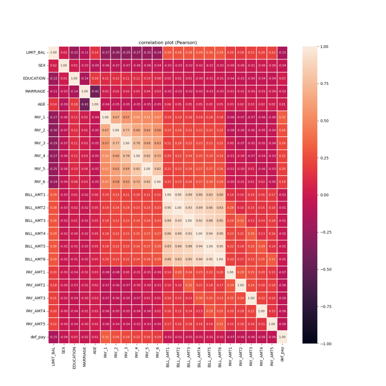
Figure 1: Heatmap of pearson correlation coefficients among feature variables

By looking at the heat map, it can be seen that PAY_1, PAY_2, PAY_3, PAY_4, PAY_5, PAY_6, and AGE have a strong correlation with def_pay, and these characteristic metrics will be analyzed in detail next (see Figure 1-4).

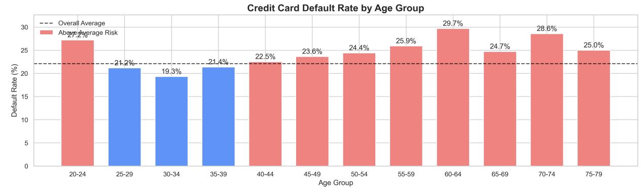
Figure 2: Default rates across various age groups

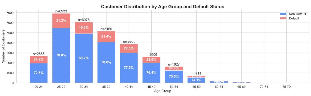
Figure 3: Distribution of default rates across various age groups

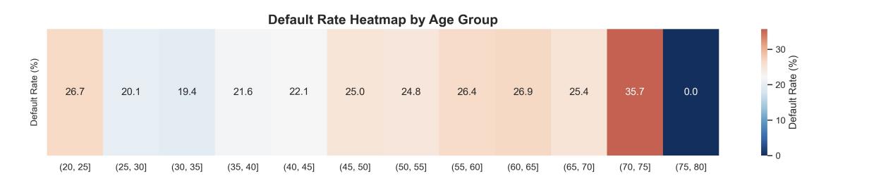
Figure 4: Heat map of default rates across various age groups

From the analysis of the chart, it can be seen that the default rate of credit card among different age groups shows a clear “U” distribution trend. The default rates of 20-24, 60-64 and 70-74 age groups are significantly higher than the overall average (about 24.2%), reaching 27.2%, 29.7% and 28.6% respectively. This trend reflects that individuals are more likely to be exposed to credit default risk at the beginning and end of their life cycle, showing a strong structural pattern.

For the younger group (20-24 years old), the higher default rate may be closely related to the fact that they are still at the beginning of their careers, have unstable incomes, and have weaker financial buffers. In addition, the financial literacy of this group is generally low, and they are prone to excessive overdrafts and neglecting repayment deadlines, which may lead to defaults. The high default rate of the older group (over 60 years old) may be influenced by multiple factors. On the one hand, retirement brings a sudden drop in income level, which may imbalance their existing debt structure; on the other hand, some elderly users may face higher pressure of medical expenses. In addition, the older population is also a high target of financial fraud, and the debt burden resulting from such fraud may also push up the default rate.

At the customer distribution level, the 25-34 age group is the main concentration of bank customers, with 6,933 and 6,078 in the 25-29 and 30-34 age groups, respectively, accounting for the highest proportion of the total sample. However, the default rates for this group are relatively low at 21.2% and 19.3%, indicating a good balance between income and debt. Customers in this age group are generally already in stable employment, have some experience in financial management, and have a lower default risk. Therefore, from the perspective of credit risk management, this group can be regarded as a “low-risk core customer group” that banks should focus on cultivating.

On the other hand, despite the relatively smaller overall number of clients aged 60 and above, with only 714 individuals in the 60–64 age group, the default rate for this group stands at an alarming 29.7%. This indicates that, although the group's size is modest, the risk exposure per account is substantial. In the event of a concentrated default, this could potentially impact the quality of the bank's assets. Consequently, in practical business operations, this demographic should be included within the scope of key monitoring (see Figure 5).

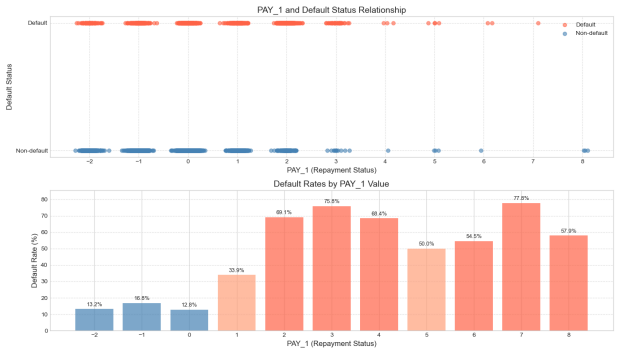
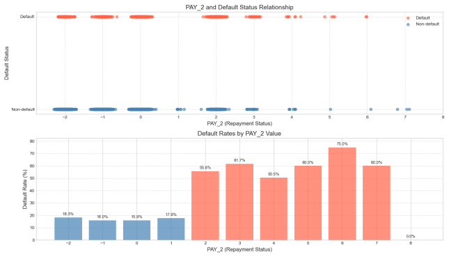
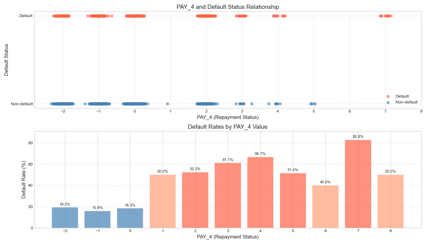
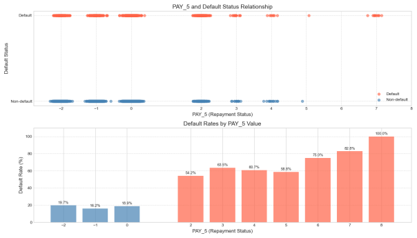
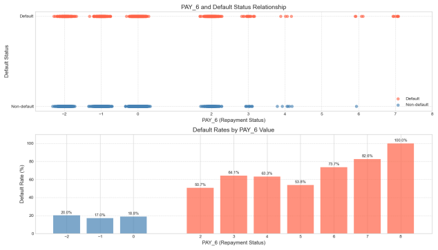
Figure 5: Repayment status and its relationship with default probability

Each of these graphs above shows the relationship between repayment status and default behavior from the first month to the sixth month in the past. It is clear from the graphs that there is a significant positive trend between the repayment status and the probability of default: i.e., the more months the repayment is delayed, the higher the probability that the borrower will default [5].

Taking PAY1 as an example, when the repayment status is normal (i.e., the value is 0 or negative), the default rate remains at a low level (<20%). However, once there is a delay in repayment (e.g., PAY1 ≥ 2), the default rate rapidly increases, reaching 75.8% when PAY1 = 3 and peaking at 77.8% when PAY1 = 7. Similarly, in the case of PAY5, the default rate has already reached 54.2% when PAY5 = 2, and it rapidly rises to over 75% when PAY5 ≥ 6, reaching a maximum of 100% when PAY5 = 8. This trend indicates that historical repayment behavior has a strong predictive power for future defaults.

This pattern has a plausible explanation in behavioural finance. First, a delay in repayment is likely to reflect the borrower's short-term cash flow constraints. If this financial constraint is not alleviated in the following months, their creditworthiness tends to deteriorate further, which in turn affects their ability to perform. Secondly, late repayment is usually accompanied by an increase in penalties and late fees, which constitutes an additional financial burden and creates an ‘interest snowball’ effect, leading to debt distress for the borrower. In addition, in the credit scoring system, consecutive late payments will significantly lower their credit rating, further limiting their ability to obtain new financing and leading them into a vicious credit cycle.

It is also noteworthy that the diagram exhibits a characteristic of "structural leap," whereby a significant increase in default rates is observed when the repayment status transitions from "non-delayed" (e.g., 0 or -1) to "minor delinquency" (e.g., 1 or 2). This indicates that even a slight delay, indicative of a minor delinquency, may serve as an early signal of deteriorating creditworthiness. Consequently, in risk control strategies, it is imperative not only to focus on high-delay customers but also to intensify monitoring of clients exhibiting incipient signs of delinquency.

In summary, all the indicators of the month's repayment status can effectively reflect the changes in the borrower's credit status, and have strong discriminatory ability. In the subsequent construction of the model, it is recommended that the monthly repayment status be considered as a core variable, especially focusing on the labeling and dynamic tracking of customers who have been overdue for many consecutive months, in order to improve the overall risk identification and early warning ability.

3. Research methodology

3.1. Method choosing

By using the decision tree method, we combined hyperparameter optimization through grid search and analysis of class weights to evaluate the performance. Decision trees offer the following advantages: high interpretability, the ability to handle non-linear relationships, the capacity to deal with missing values and outliers, feature selection and importance assessment, and fast model training and prediction. They are highly suitable for the characteristics of bank credit datasets.

Traditional decision tree models are based on features and recursively partition the sample space. When dealing with complex data, their generalization ability is poor. For example, when there are complex non-linear relationships among data features, decision trees may not accurately capture them, resulting in sub - optimal performance on the test set. Moreover, for imbalanced class data, they tend to be overly biased towards majority-class samples and overlook the features of minority-class samples. In credit default prediction, this might lead to an underestimation of default risks. Additionally, the selection of hyperparameters often relies on experience, lacking systematic optimization, which makes it difficult to fully unleash the model's potential [6].

3.2. Feature engineering

In the dataset, the default rate of the male group is relatively high, and the default rate of the married group is also relatively high. In order to facilitate data processing and improve the efficiency of the model, in terms of feature engineering, a category for married men, a combined category for married women and single men, a category for "divorced" men, a category for single women, and a category for "divorced" women are created: 1 #married man, 2 #single man, 3 #divorced man, 4 #married woman, 5 #single woman, 6 #divorced woman. Since there is too little data for divorced women, which may affect the results of the model, we choose to exclude divorced women.

3.3. Concrete procedure

When using decision trees to analyze a bank's credit risk dataset, the first step is to comprehensively gather relevant data such as customers' basic information, financial status, and credit history. Thoroughly understand the characteristics of this data and the distribution of credit risks. Subsequently, initiate data cleaning, dealing with missing values and outliers. After encoding the features, divide the dataset into subsets at an appropriate ratio.

Build a basic decision tree model and conduct an initial training. To address the issue of class imbalance, set class weights. Define the ranges for hyperparameters, including tree depth, the minimum number of samples required to split an internal node, and the minimum number of samples required to be at a leaf node. Employ grid search to iterate through all possible combinations and use cross-validation for evaluation. Select the optimal hyperparameters based on the results [7].

Train the final model using these optimal hyperparameters. Evaluate the performance of the model on the test set using multiple metrics, including accuracy, precision, recall, F1-score, and ROC-AUC. Leverage the interpretability of the decision tree to analyze the importance of features and optimize the model accordingly.

Finally, deploy the model and continuously monitor it. Update the model in a timely manner according to new data and business requirements to ensure that it can accurately predict credit risks. Comparison of decision trees with different depths: For the decision tree model with a depth of 2, the accuracy rate reaches 0.820, and the F1-score is 0.425. For the decision tree with a depth of 3, the accuracy rate slightly increases to 0.821, and the F1-score rises to 0.470. While for the decision tree with a depth of 5, the accuracy rate is 0.817, and the F1-score is 0.453. This indicates that within a certain range, as the depth of the decision tree increases, there are some fluctuations in the accuracy rate and F1-score of the model, but the overall change is not particularly significant. However, when the depth increases to 5, both the accuracy rate and the F1-score decrease compared to when the depth is 3, which shows that an overly deep decision tree may suffer from overfitting, leading to worse performance on the test set. The default model with grid search tuning: The accuracy rate of the "Grid Search Tuned (Default)" model is 0.761, and the F1-score is 0.508. Compared with the decision tree models with different depths, its accuracy rate is significantly lower, indicating that the parameters tuned by default may not have adapted well to the data, resulting in poor model performance. The F1 - score of this model is quite high. This might mean that it has achieved a relatively balanced result between the recall rate and the precision rate[8].

In the models tuned by grid search, both those with and without class weights. First, consider the "Grid Search Tuned (No Class Weight)" model. Its accuracy rate is the same as that of the decision tree model with a depth of 3. They are both 0.821. Also, its F1-score is equal to that of the decision tree model with a depth of 3. The F1-score is 0.470. This shows that when no class weight is set, the performance of this model is similar to that of the decision tree model with a specific depth.

Next, take a look at the "Grid Search Tuned (With Class Weight)" model. Its accuracy rate is 0.851, and its F1-score is 0.585. Among all the models, it has the highest accuracy rate and F1-score. In addition, this indicates that when dealing with imbalanced class data, setting class weights can effectively improve the performance of the model. The model becomes more accurate in predicting credit risks. It not only improves the ability to identify positive cases (such as customers who default) but also keeps the overall accuracy rate high.

Finally, we still used models such as logistic regression, decision tree, and SVM to compare their performance [9]. The results are as follows (see Table 2).

Table 2: Results of different models

In this comparison of model performance, each model exhibits distinct characteristics. The logistic regression model has an accuracy of 0.75 and an F1-score of 0.55. It features a low level of complexity, with a relatively simple structure. However, it is highly sensitive to data imbalance. There is a certain potential for performance improvement through parameter tuning. The decision tree model showcases remarkable advantages. With an accuracy as high as 0.92 and an F1-score of 0.65, it stands out among the various models. It can handle data in a clear and intuitive tree-like structure, demonstrating a strong ability to capture complex data patterns. Even though its model complexity is evaluated as low, it can still efficiently explore the relationships among data features and complete classification tasks with high precision. Nevertheless, the decision tree is quite sensitive to data imbalance. By performing pruning operations, its performance can be further optimized, reducing the risk of overfitting. The random forest model has an accuracy of 0.72 and an F1-score of 0.50. Its model complexity is at a moderate level, and so is its sensitivity to data imbalance. Thanks to its built-in balancing mechanism, it possesses significant potential for performance enhancement. The SVM (Support Vector Machine) model has an accuracy of 0.70 and an F1-score of 0.40. It has a high level of model complexity. Although it has a low sensitivity to data imbalance, improving its performance heavily relies on sampling and is rather challenging [10].

4. Conclusion

Through this study, the decision tree model demonstrates the most comprehensive performance in credit default prediction. As financial markets accelerate their digital transformation, data dimensions and volumes continue to grow.

In response to the shortcomings of traditional decision tree models, hyperparameter optimization is carried out through grid search, and class weights are set to address the issue of class imbalance. This effectively improves the performance of the model, enabling it to perform better when dealing with complex and imbalanced data.

Future research could incorporate diverse data types, such as borrowers' consumption behavior patterns, social media activity information, and others, to develop more diverse and comprehensive models. This would enable more precise capture of credit risk characteristics and enhance the accuracy and foresight of risk assessments.

Model interpretability remains critical in the financial sector. Future efforts should focus on developing advanced visualization tools to illustrate the decision-making processes of complex models, aiding financial institutions in understanding model logic and strengthening trust in model outcomes.In practical applications, establishing real-time monitoring and dynamic updating systems is essential. Such systems could continuously track borrowers' credit status, promptly adjust risk evaluation results, and adapt to market fluctuations in real time, providing immediate decision-making support for financial institutions.

Regarding cross-industry applications, the findings of this study could be extended to fields such as supply chain finance and consumer finance. By tailoring models to industry-specific characteristics, machine learning can be widely adopted in financial risk management, fostering stable development across the financial sector.

Authors contribution

All the authors contributed equally and their names were listed in alphabetical order.

References

[1]. Wang, Z. Q. (2025)Does Digital Transformation Amplify Credit Risks in Commercial Banks?China Knowledge Network.
[2]. Ken Brown ,Peter Moles.(2014)Credit Risk Management: Methods, Models, and Tools. EBS Online.
[3]. Sun G., Wang Y.¹, Li Q.,(2022) School of Economics, Dongbei University of Finance and Economics, School of Economics, Nanjing University of Finance and Economics, The Impact of Green Credit on Commercial Bank Credit Risk.China Knowledge Network.
[4]. Gross, J. P. K., Cekic, O., Hossler, D., & Hillman, N. (2021)What matters in student loan default: A review of the literature. Journal of Student Financial Aid, 39(1), 19–29.
[5]. Zhao, Y., (2021) Research on Credit Default Prediction Based on Fusion Model and Feature Importance AnalysisJ. Data. 2021, 202103: 62-64.
[6]. Breiman, L. (2001). Random forests. Machine Learning, 45(1), 5-32.
[7]. Hastie, T., Tibshirani, R., & Friedman, J. H. (2009). The Elements of Statistical Learning. Springer,2, 44-47.
[8]. Breiman, L., Friedman, J. H., Olshen, R. A., & Stone, C. J. (1984). Classification and Regression Trees. Wadsworth & Brooks/Cole.
[9]. Chawla, N. V., Bowyer, K. W., Hall, L. O., & Kegelmeyer, W. P. (2022). SMOTE: Synthetic minority over-sampling technique. Journal of Artificial Intelligence Research, 16, 321-357.
[10]. Vapnik, V. N. (1995). The Nature of Statistical Learning Theory. Springer, 5, 105-108.
Cite this article
Gan,Y.;Luo,H.;Wei,W. (2025). Credit Risk Management Based on Decision Tree Model. Advances in Economics, Management and Political Sciences,185,84-92.
Data availability
The datasets used and/or analyzed during the current study will be available from the authors upon reasonable request.
Disclaimer/Publisher's Note
The statements, opinions and data contained in all publications are solely those of the individual author(s) and contributor(s) and not of EWA Publishing and/or the editor(s). EWA Publishing and/or the editor(s) disclaim responsibility for any injury to people or property resulting from any ideas, methods, instructions or products referred to in the content.
About volume
Volume title: Proceedings of ICEMGD 2025 Symposium: Innovating in Management and Economic Development
© 2024 by the author(s). Licensee EWA Publishing, Oxford, UK. This article is an open access article distributed under the terms and
conditions of the Creative Commons Attribution (CC BY) license. Authors who
publish this series agree to the following terms:
1. Authors retain copyright and grant the series right of first publication with the work simultaneously licensed under a Creative Commons
Attribution License that allows others to share the work with an acknowledgment of the work's authorship and initial publication in this
series.
2. Authors are able to enter into separate, additional contractual arrangements for the non-exclusive distribution of the series's published
version of the work (e.g., post it to an institutional repository or publish it in a book), with an acknowledgment of its initial
publication in this series.
3. Authors are permitted and encouraged to post their work online (e.g., in institutional repositories or on their website) prior to and
during the submission process, as it can lead to productive exchanges, as well as earlier and greater citation of published work (See
Open access policy for details).