1. Introduction

The global economy is undergoing rapid digital transformation, with financial technology evolving continuously. As a result, the credit market has experienced explosive growth in recent years, and China's personal credit industry has entered the digital era [1]. The rise of online lending not only addresses the demand for small loans but also stimulates the economy and complements the traditional credit market. However, many lending institutions, in pursuit of high profits, fail to recognize the uncontrollable relationship between borrowers' characteristics and defaults, overlooking potential risks that lead to credit defaults. In today's era of big data, credit default risk has become a significant concern for financial institutions. Traditional decision-making methods, combining manual processing and machine approval, have become outdated. Therefore, building a reliable prediction model to address this issue has become essential [2].

Previous research has shown that traditional machine learning and statistical methods often fail to fully exploit data, resulting in predictions that are generally less accurate compared to machine learning and deep learning-based models [3]. To better mine data features and reduce default risk, this study utilizes loan data from LendingClub, a leading P2P lending platform in the U.S., covering the period from 2007 to 2015, for default prediction. After comparing various data features, the Gradient Boosting Decision Tree (GBDT) model under integrated boosting is selected to explore the relationship between variables and identify the factors most influential in default. The machine learning models used for comparison include Logistic Regression, Decision Tree Classifier, Random Forest Classifier, Gradient Boosting Classifier, and XGBoost Classifier. To further optimize the models, several data balancing techniques, such as SMOTE, ADASYN, Random Over Sampler, Random Under Sampler, SMOTEENN, and SMOTETomek, are applied.

This study employs a series of tree-based learning models, drawing from previous research, to provide a more reliable method for default prediction. These models effectively identify key features of defaults, enhancing prediction accuracy, improving credit risk management, and contributing to the development of the financial economy.

2. Related principles and techniques

2.1. Gradient boosting

GBDT is a tree model based on Boosting algorithm. It consists of multiple decision trees and the model is continuously optimised through iterative training. First, a positive value is assigned to the sample prediction. In the first iteration, the first tree adjusts the initial value by calculating the negative gradient of the current model's loss function, which becomes the new target value. Then, the next decision tree is trained to fit that negative gradient. The output of the new tree is added to the existing model output to update the model. This process continues, and finally, the results of all the decision trees are accumulated to obtain the prediction [4]. In contrast to traditional Boosting GBDT does not need to update the sample weights significantly. But it indirectly achieves a focus on difficult samples by fitting negative gradients to focus on samples that are poorly predicted by the current model.

2.2. Random oversampling

Random Oversampling is a technique applied to deal with the problem of category imbalance in a dataset, and it is the most direct and effective method for imbalanced data. It improves the model's ability to learn and predict the minority class by randomly selecting more samples from the minority class. This creates a more balanced distribution of classes in the dataset, achieving a sample ratio of 1:1 in each class, which enhances the model's ability to learn and predict the minority class [5].

3. Data exploration and analysis

3.1. Data acquisition and description

The lending club dataset derived from kaggle was selected for this study. This dataset collects lending information from 2007 to 2015 and filters out some irrelevant features to provide relevant information related to the borrower. This is a two-dimensional data containing 14 features, 9578 samples, and the target variable not fully paid, where 0 represents a non-defaulting user and 1 represents a defaulting user. The dataset has many types of features, and there is a nonlinear relationship between some features, and there are outliers in the dataset. The tree model can effectively implement the classification and regression problems. It has a good fit to the data, and can tap into the complex non-linear relationships between features [6]. The next study will be based on a series of tree-related models for training (see Table 1).

Table 1: Description of each feature

3.2. Data pre-processing

For the categorical variables in the data, they need to be converted into numerical variables for analysis in order to facilitate the use of subsequent predictive models. And in this study, all variables were unified into numerical variables using label coding. Based on the characteristics of the data, it can be seen that there are no missing values in this dataset, which do not need to be processed. In order to make the model training more accurate, the outliers present in the data need to be mined. Outliers refer to values in the dataset that deviate from the normal range. And although the overall percentage is small, they can lead to overfitting problems that have an impact on subsequent research [7]. In this study, the outliers were replaced with mean values to arrive at reasonable data.

4. Feature screening and analysis

4.1. Feature selection

After the initial processing of the data, the important features need to be further analysed in order to accurately analyse the possible factors of default. Feature screening based on feature importance is widely applied in machine learning. In this paper, based on the description of the dataset, the initial screening of features is done based on the GBDT model.

As shown in the Figure 1 below, four features, int.rate,fico,inq.last.6mths,installment, are selected from it, and they will be analysed in detail with the knowledge of economics next.

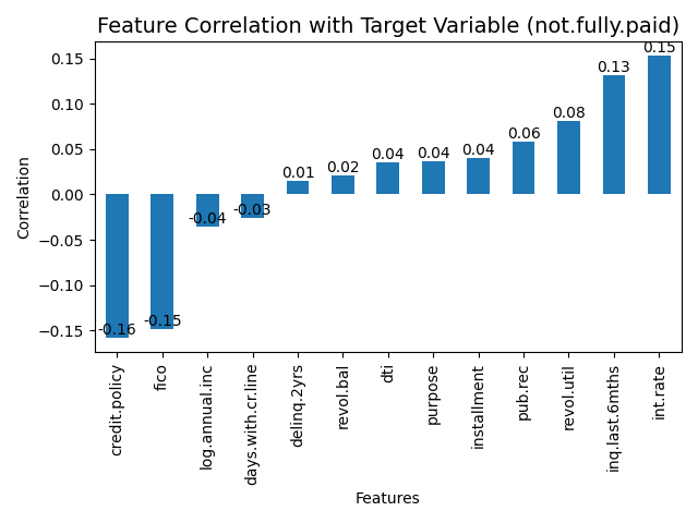
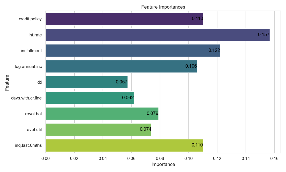
Figure 1: Correlation between variables and target variables

The following Table 2 shows the mean, minimum, maximum, skewness and kurtosis of the significant features. The study will analyse these metrics in conjunction with the images.

Table 2: Description of important feature data

(i) int.rate (loan interest rate)

The majority of loans have interest rates concentrated around 0.12. And the distribution of interest rates on loans that are not fully paid has two peaks, one around 0.08 and the other around 0.12. The distribution of interest rates on loans that are fully paid is concentrated around 0.12 and has a more concentrated distribution. The low-interest rate loans in the Figure 2 may have attracted more high-risk borrowers because they had easier access to loans. But they were less able to repay them, leading to higher default rates. Higher interest rate loans may themselves be aimed at higher risk borrowers and therefore also have higher default rates.

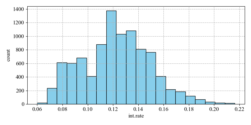
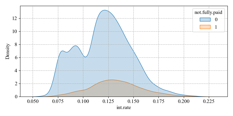
Figure 2: Distribution of int.rate

(ii) inq.last.6mths (the number of times the borrower has been queried in the last six months)

The mean value is 1.577469, the minimum value is 0, the maximum value is 33, while the skewness is 0.993807. This indicates an overall right skewness, uneven data distribution, and a large difference in the number of times a borrower has been queried among borrowers. A higher number of enquiries may indicate that the borrower has a high risk of default due to a high demand for funds in the near future. A lower number of enquiries means that the borrower does not need to go through multiple approvals and has a lower risk of default.

In the Figure 3, being in a position where there are fewer times of being queried, e.g. 0 times to near the mean, the number of non-defaults is much higher than the number of defaults. This distinction can be well differentiated as a way to improve the prediction accuracy.

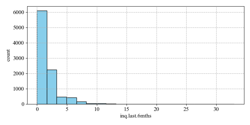
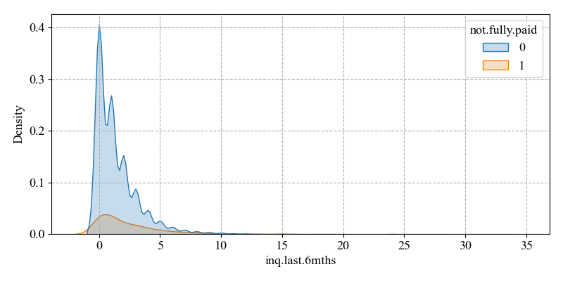
Figure 3: Distribution of inq.last.6mths

(iii) Fico(credit score)

The mean is 710.8463 with a maximum value of 827 and a minimum value of 612, while the skewness is 0.414160. It indicates that the majority of the sample is to the right of the mean and is right skewed. High credit scores are usually perceived to have lower default rates and correspondingly low credit scores are perceived to have higher default rates.

The number of non-defaults is much higher than the number of defaults for borrowers whose ranges are on the right side of the mean. The implication is that it is possible to distinguish non-defaults from defaults on the right side of the mean, thus detecting default status and improving prediction accuracy. Credit scores directly affect the level of interest rates on loans. High credit scores usually result in lower loan interest rates and a lower risk of default. Borrowers with low credit scores may face greater loan stress and higher risk of default (see Figure 4).

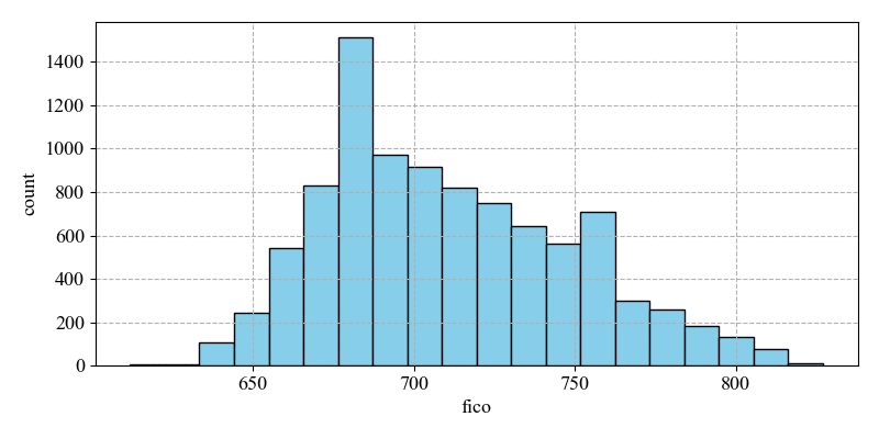
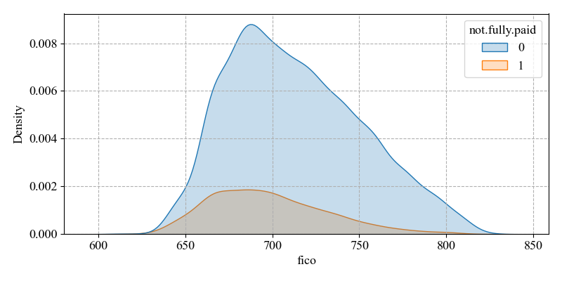
Figure 4: Distribution of fico

(iv) Installment (monthly installments owed by the borrower)

The mean value is 319.0894, the maximum value is 910.14, and the minimum value is 15.67, while the skewness is 1.641318. It indicates that a large number of samples are on the right side of the mean, with the overall right skewness. And the difference between the maximum and the minimum value is large, and the data are not evenly distributed. The higher the instalment, the higher the repayment pressure the borrower has to bear and the higher the risk of default.

As the number of non-defaults is much higher than the number of defaults on the left side of the graph's mean. The range can be well delineated between non-defaults and defaults status, thus improving the prediction accuracy (see Figure 5).

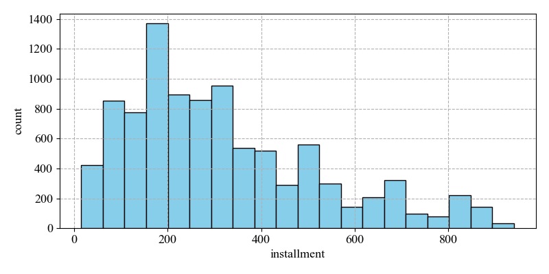
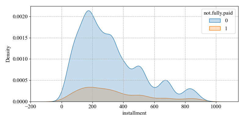
Figure 5: Distribution of installments

4.2. Correlation analysis

Correlation analysis focuses on the analysis between two or more variables to illustrate the relationship that exists between two variables. It is a measure of the closeness between phenomena and a representation of the relationship that exists for a phenomenon [8]. According to the correlation coefficients of the features demonstrated by the heat map, the darker the colour the stronger the correlation and the lighter the correlation the weaker the correlation. Most of the features do not have a strong correlation with each other. While the correlation between int.rate and fico is stronger and reaches 0.74. Therefore, the correlation is retained and analysed with knowledge of economics.

Interest rates are more related to credit risk. When granting loans, financial institutions will use credit scores to predict the default risk of borrowers and use this as a basis for adjusting loan interest rates. For borrowers with high credit scores, financial institutions will compete to lower interest rates to attract them to choose their own loan products. As these people have a strong repayment ability and willingness to pay back the loan, and the risk of default is lower. For borrowers with low credit scores, in order to avoid losses from defaults, financial institutions may raise loan interest rates while imposing restrictions on loan modes and repayment amounts. And as the real interest rate rises, the real value of the borrower's debt tends to increase, the greater the pressure that needs to be borne on the loan, which makes the debt repayment cost higher and increases the possibility of loan default [9].

Of course, borrowers with high credit scores may also face high interest rates. When the economy is tough and financial institutions are faced with a cash crunch, they will raise the interest rates on their loans. Whereas borrowers with low credit scores who can repay their loans on time over a period of time, proving that their repayment ability and credit scores have improved. Financial institutions will lower their loan interest rates appropriately (see Figure 6).

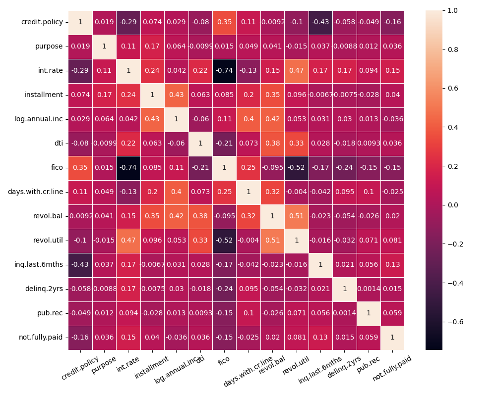
Figure 6: Correlation heat map

5. Modelling experiment

5.1. Data set division

This experiment is divided into training set data and test set data in the ratio of 4:1. The training set data is for model training and data balancing processing. The test set data is used for performance evaluation and comparison after the model training is completed.

5.2. Indicators for model evaluation

The results of the model evaluation will be analysed in relation to the metrics AUC, accuracy, F1-score, recall, and precesion.

(i) Accurcy: It is the ratio of the number of samples predicted accurately to the total number of samples, and is a basic indicator for evaluating the goodness of a classification model. Accurcy evaluates the overall prediction ability of the model, the higher the accuracy, the better the model is.

(ii) Precision: It reflects the accuracy of the model's prediction results, the higher the accuracy, the better the prediction.

(iii) Recall: It represents the proportion of all actual defaults that are predicted to be defaults, and the recall rate is the ratio of correctly predicted defaults to all actual defaults.

(iv) Fl-Score: This is calculated based on precision and recall, and combines the two indicators to reflect the evaluation capability of the model.

(v) AUC: It is the area under the ROC curve, which is employed to measure the performance of a binary classification model. The closer the AUC value is to 1, the better the model performance is; the closer it is to 0.5, the worse the model performance is.

5.3. Model training and comparison

The study is based on LogisticRegression, DecisionTreeClassifier, RandomForestClassifier, GradientBoostingClassifier, XGBoost, AdaBoost, Bagging, which are several machine learning models. Evaluated using AUC, precision, recall, f1-score, accuracy metrics.

Based on the data from the model training, it can be seen that the performance ranking of each model is as follows in Table 3.

GradientBoostingClassifier >AdaBoost >RandomForestClassifier >LogisticRegression >XGBoost >Bagging >DecisionTreeClassifier. The model overall is more accurate for data mining. The GBDT model has the highest AUC value and better overall performance. Comparing the other models, the results are better in terms of accuracy in class 0, 1 training, both of which have a certain degree of recognition. Although there is only 0.04 in class 1 recall, there is still room for improvement. Therefore the following will be a series of studies around GBDT.

Table 3: Comparison chart of model training

6. Data balancing

Defaults account for 84 per cent of this data and non-defaults for 16 per cent, giving a positive to negative sample ratio of 5:1 and a class imbalance. Class imbalance refers to the uneven distribution of classes in the training set used in training the classifier. In order to solve this problem, a data balancing approach is needed to adjust the degree of sample imbalance [10]. The study was conducted using SMOTE, ADASYN, RandomOverSampler, RandomUnderSampler, SMOTEENN, and SMOTETomek, which were trained based on different models. Combining the AUC, f1 value, accuracy, recall and other metrics, it was discovered that RandomOversampling outperformed the other methods in all these aspects. Failed to improve on AUC, but improved on Class 1 recall and maintained good overall performance.

Next train again with the selected GBDT model based on the random oversampling algorithm. The random_state was set to 0 when dividing the dataset before the experiment to ensure that each run was performed on the training set and the same random results were obtained (see Table 4).

Table 4: Comparison of performance before and after balancing

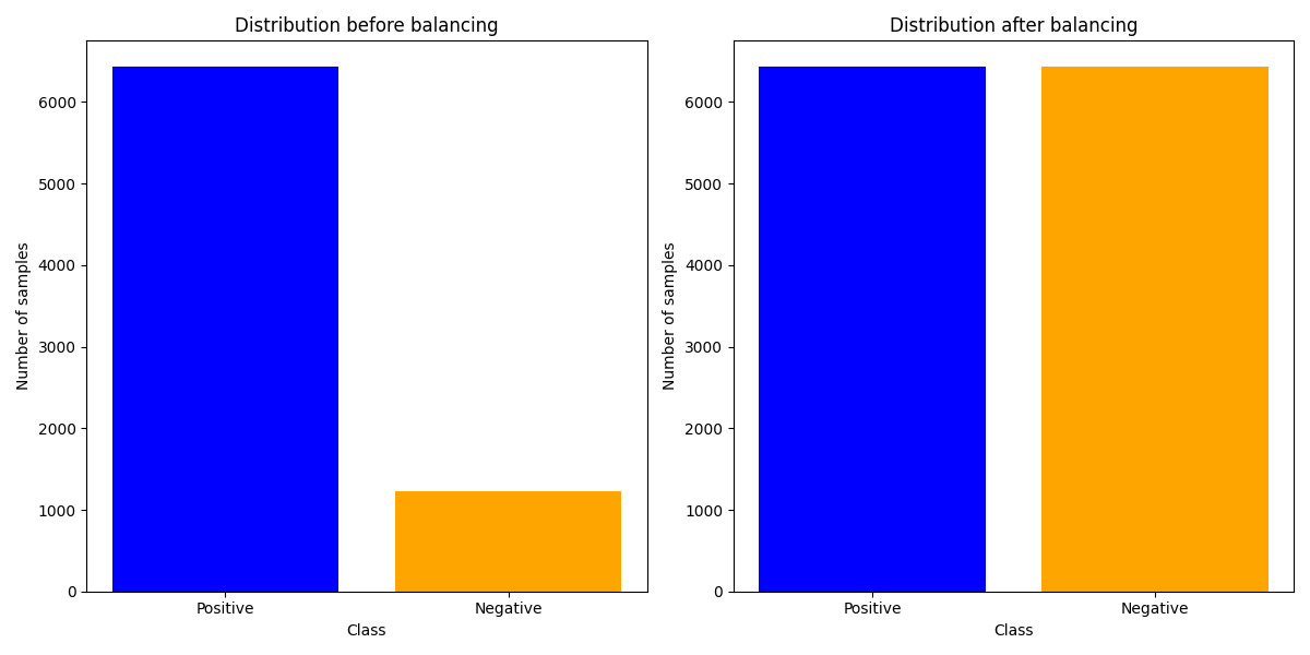
Figure 7: Percentage of positive and negative samples before and after balancing

According to the data before and after balancing presented in the table 4 and the percentage of positive and negative samples in the figure 7 the ratio of positive and negative samples before training is 5:1, while after training the ratio is 1. It is shown that RandomOversampling has the effect of balancing the data by replicating the samples for fewer classes. The Class 1 recall rate increased from 0.04 to 0.410, an improvement of 926 per cent, allowing for better identification of default status compared to before (see Figure 7).

7. Conclusion

This paper focuses on predicting credit default risk using data from LendingClub between 2007 and 2015, analyzing the most relevant features. After splitting the dataset into training and test sets, various machine learning models were applied, trained, and compared. The data was then balanced using different techniques to optimize the model. The study not only examines the feasibility of the model but also provides a detailed explanation of the relevant features and model selection. The key findings are as follows:

First, descriptive statistics of the dataset reveal that factors such as loan interest rate, the number of times the borrower was queried in the last six months, credit score, and monthly installments owed have a significant impact on the target variables, with strong predictive power for defaults. Notably, there is a high correlation between loan interest rate and credit score. Second, after training seven models (Logistic Regression, Decision Tree Classifier, Random Forest Classifier, Gradient Boosting Classifier, XGBoost, AdaBoost, and Bagging). It was found that the Gradient Boosting Classifier performed best on the data. This model served as the basis for data balancing. Balancing the data using methods like SMOTE, ADASYN, RandomOverSampler, RandomUnderSampler, SMOTEENN, and SMOTETomek, it was determined that RandomOverSampler offered the best overall balance. Although the AUC value did not show improvement, there was a significant increase in recall for class 1.

Furthermore, this study focused exclusively on tree-based models based on the features in the dataset. Other models were not considered, and some potentially important factors were excluded, resulting in a relatively limited number of features. Future research can explore additional models and data balancing techniques to further optimize the results. Additionally, experiments involving datasets with a broader range of features could help identify other factors influencing defaults and improve the accuracy of credit default predictions.

References

[1]. Ma W.M., (2024) Credit Default Prediction Based on k-Stratified SMOTE-CV with Stacking Integrated Learning. Intelligent Computers and Applications, 14, 146-152.
[2]. Cai Q.S., Wu J.D., Bai C.Y., (2021) Credit Default Prediction Based on Interpretable Integration Learning. Computer System Applications,30(12), 194–201.
[3]. Zhang J., ,(2022)Research on Bank Credit Customer Default Risk Prediction Based on Integrated Learning Models. Chengdu University of Technology. DOI:10.26986/d.cnki.gcdlc.2022.000890.
[4]. Wang X.Y., (2020) Research on Big Data Risk Control Model Based on GBDT Algorithm.Journal of Zhengzhou Aviation Industry Management College,38(05), 108-112.DOI:10.19327/j.cnki.zuaxb.1007-9734.2020.05.009.
[5]. Gao Y.J., (2023) Research on Credit Default Prediction Based on Optimal Base Model Integration Algorithm. Intelligent Computers and Applications,13(07), 64-70+75.
[6]. Luo Z.A., (2021) Research on Stacking Quantitative Stock Picking Strategy Based on Integrated Tree Modelling. Chinese Prices, 02, 81-84.
[7]. Lai W.B., (2023) Research on P2P Credit Default Prediction Based on CatBoost Stacking Approach. Jiangxi University of Finance and Economics. DOI:10.27175/d.cnki.gjxcu.2023.000789.
[8]. Wang S.Y., Cao Z.F., Chen M.Z., (2016) A study on the Application of Random Forest in Quantitative Stock Selection. Operations Research and Management,25(03), 163-168+177.
[9]. Asror N., Syed S., Khorshed A., (2022) Macroeconomic Determinants of Loan Defaults: Evidence from the U.S. peer-to-peer lending market. Research in International Business and Finance, Volume 59, 101516. ISSN 0275-5319,https://doi.org/10.1016/j.ribaf.2021.101516.
[10]. Liu B., Chen K., (2020) A Loan Risk Prediction Method Based on SMOTE and XGBoost. Computers and Modernisation,2, 26-30.
Cite this article
Luo,C. (2025). GBDT-Based Credit Default Prediction. Advances in Economics, Management and Political Sciences,170,77-86.
Data availability
The datasets used and/or analyzed during the current study will be available from the authors upon reasonable request.
Disclaimer/Publisher's Note
The statements, opinions and data contained in all publications are solely those of the individual author(s) and contributor(s) and not of EWA Publishing and/or the editor(s). EWA Publishing and/or the editor(s) disclaim responsibility for any injury to people or property resulting from any ideas, methods, instructions or products referred to in the content.
About volume
Volume title: Proceedings of the 9th International Conference on Economic Management and Green Development
© 2024 by the author(s). Licensee EWA Publishing, Oxford, UK. This article is an open access article distributed under the terms and
conditions of the Creative Commons Attribution (CC BY) license. Authors who
publish this series agree to the following terms:
1. Authors retain copyright and grant the series right of first publication with the work simultaneously licensed under a Creative Commons
Attribution License that allows others to share the work with an acknowledgment of the work's authorship and initial publication in this
series.
2. Authors are able to enter into separate, additional contractual arrangements for the non-exclusive distribution of the series's published
version of the work (e.g., post it to an institutional repository or publish it in a book), with an acknowledgment of its initial
publication in this series.
3. Authors are permitted and encouraged to post their work online (e.g., in institutional repositories or on their website) prior to and
during the submission process, as it can lead to productive exchanges, as well as earlier and greater citation of published work (See
Open access policy for details).