1. Introduction

With the improvement of people's quality of life and the continuous expansion of the scale of credit, the proportion of credit in commercial banks and other financial institutions is increasing, on the one hand, the popularity of credit cards has brought about the growth of personal credit demand, such as consumer credit, housing credit. Enterprise development has led to an increase in the demand for corporate loans, which has brought new opportunities to the banking industry. On the other hand, the expansion of credit scale brings potential risks [1]. According to the People's Bank of China's 2022 Financial Stability Report, the non-performing loan ratio of banking financial institutions is 1.80%, and the overall non-performing loans have increased. This will affect the development of banks and other financial institutions themselves, and even affect the entire financial system and economy. In the face of this problem, financial institutions need accurate credit default prediction that can help financial institutions identify potential risks in advance, rationally allocate credit resources, and reduce default losses [2]. Traditionally, credit defaults have been based on the customer's past history, but the information is often less comprehensive and detailed [3]. Through data technology, different factors are divided into bank risk data, so as to analyze and predict potential risks and customers [4]. It is found that the machine learning model can handle credit default prediction better than the traditional model [5].

At present many scholars have carried out research in the field of credit defaultprediction. Although logistic regression is widely used in this field, it has no obvious advantages over other complex models, and Probit and logistic regression mainly rely on linear relationships to process datasets, and their ability to capture feature interactions is limited [6]. Belma Ozturkkal uses the Shap-Lasso combination to model mortgage projects, but there are some problems with the lack of relevant data, which has an impact on the model performance [7]. LightGBM can handle nonlinear relationships, and the LightGBM model optimized by Bayesian method can better handle the problem of credit default prediction, but it performs poorly on abnormal data [8]. Many studies have used Xgboost as a predictive model, especially in the financial field, and as a powerful ensemble learning algorithm, it has shown strong performance in handling classification tasks [9,10]. The purpose of this paper is to develop a more accurate and effective credit default prediction model, so as to provide financial institutions with a more valuable basis for decision-making and improve their risk management level. In the face of data set imbalance, this study adopts the SMOTE method to effectively solve the problem of data imbalance and improve the performance of the model. In terms of model selection, the performance difference between LightGBM and XGBoost is compared, so as to predict credit risk.

2. Data processing

The dataset in this paper uses the credit_risk dataset on the Kaggle platform, which covers characteristic variables: borrower age, annual income, home ownership, years of employment, loan intention, loan grade, loan amount, interest rate, loan income percentage, historical default, and credit history length, and the target variable is whether the lender defaults. The sample size was 390972 and 11 characteristic variables, including 4011 missing values, all of which were filled with medians, with 0 in Table 1 representing no missing values, and 895 and 3116 representing the number of missing values in the years of employment and loan interest rate, respectively.

Table 1: The number of missing values

2.1. The data is unbalanced

As can be seen from Table 2 and Figure 1, this dataset contains 78% non-defaults and 22% defaults. In order to solve the problem of data imbalance, SMOTE is used to reduce the risk of overfitting the model in the face of new data, improve the detection ability of the model in practical applications, and promote the recall rate of the model, so as to meet the purpose of this project to capture more non-defaulters in the prediction. (0 means that the customer is not in default, 1 means that the customer is in default)

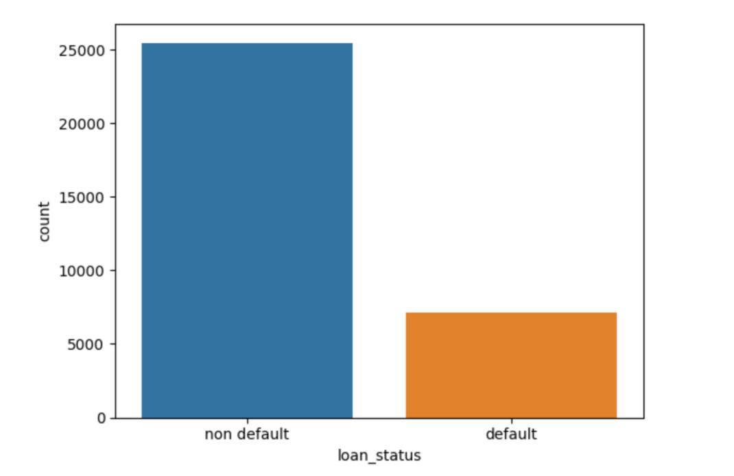
Figure 1: The percentage of customers who are in default

Table 2: The percentage of customers who are in default

2.2. Models and their theoretical underpinnings

2.2.1. SMOTE

SMOTE is one of the main methods to deal with sample imbalance, in the feature space of a minority sample, for each sample xi, find k neighbors near it, and randomly select a sample xj in it, generate a new sample, and finally interpolate in the feature space, and repeat the above process continuously to achieve equilibrium in the sample number, the formula is as follows.

\( {x_{new}}={x_{i}}+λ\cdot ({x_{i}}-x) \) (1)

2.2.2. XGBoost model

XGBoost, as a representative of ensemble learning, is an efficient gradient boosting framework, which continuously corrects the error of the previous decision tree and the residuals of the previous decision tree of the subsequent order of the decision tree, and finally weights the prediction results of the total number of trees set. Here is the core formula of XGBoost, which is divided into the following three parts:

The first part is the regularized objective function, which consists of a loss function and model complexity:

\( L(Θ)=\sum _{i=1}^{n}L({y_{i}},\hat{y}_{i}^{(t-1)}+{f_{t}}({x_{i}}))+γT+\frac{1}{2}λ\sum _{j=1}^{T}w_{j}^{2}\hat{y}_{i}^{(t-1)} \) (2)

\( \hat{y}_{i}^{(t-1)} \) is the cumulative predicted value of the previous t−1 tree, \( {f_{t}} \) is the cumulative predicted value of the previous t−1 tree, \( T \) is the number of leaf nodes, \( {w_{j}} \) is the weight of the leaf nodes, and \( γ \) and \( λ \) are the regularization hyperparameters.

The second part is a second-order Taylor expansion approximation of the loss function:

\( {L^{(t)}}≈\sum _{i=1}^{n}[{g_{i}}{f_{t}}({x_{i}})+\frac{1}{2}{h_{i}}f_{t}^{2}({x_{i}})]+Ω({f_{t}}) \) (3)

These \( {g_{i}}={∂_{{\hat{y}^{(t-1)}}}}L({y_{i}},{\hat{y}^{(t-1)}}) \) \( {h_{i}}=∂_{{\hat{y}^{(t-1)}}}^{2}L({y_{i}},{\hat{y}^{(t-1)}}) \) are the first- and second-order gradients of the loss function, respectively.

The third part is the tree structure generation and classification criteria:

\( Gain=\frac{1}{2}[\frac{{(\sum _{i∈{I_{L}}}^{​}{g_{i}})^{2}}}{\sum _{i∈{I_{L}}}^{​}{h_{i}}+λ}+\frac{{(\sum _{i∈{I_{R}}}^{​}{g_{i}})^{2}}}{\sum _{i∈{I_{R}}}^{​}{h_{i}}+λ}-\frac{{(\sum _{i∈I}^{​}{g_{i}})^{2}}}{\sum _{i∈I}^{​}{h_{i}}+λ}]-γ \) (4)

In Equation (4), \( {I_{L}} \) and \( {I_{R}} \) are the sample sets of the left and right subnodes after splitting, respectively, and the gain calculation combines the loss reduction and complexity penalty.

3. Analysis of experimental results

3.1. Correlation of the characteristic variable with the target variable

From the correlation graph (Figure 2), it can be seen that there are a total of 11 characteristic variables, namely the ratio of loan to income, loan grade, interest rate, home ownership, historical default history, personal annual income and loan amount, and whether the customer defaults or not is the target variable. (In this paper, the characteristic variables of corr>0.1 are selected for specific analysis).

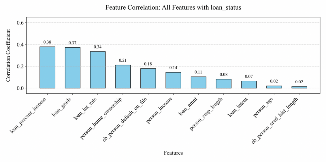
Figure 2: Correlation between target variables and characteristic variables

3.2. Discrete data analysis (corr>0.1 data)

As can be seen from Figure 3 and Table 3, most of the defaults are A-D (A-G risk increases), and in terms of proportion, about 83% of defaulting renters have loans rated A, B, or C. From the perspective of sample size, financial institutions such as general banks with scale effects and low risk ratings are more likely to lend, so the number of A-D grades is relatively large. (0 and 1 represent that the customer has not defaulted and the customer has defaulted respectively)

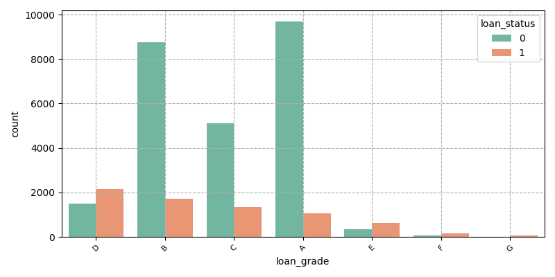
Figure 3: Credit rating

Table 3: Proportion of different credit ratings

As can be seen from Figure 4, most of the loan defaulters are renters, and the general renters have large job changes, poor income stability, and limited accumulated funds. (0 and 1 represent that the customer has not defaulted and the customer has defaulted respectively)

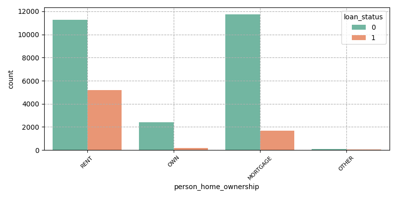
Figure 4: Home ownership

As can be seen from Figure 5, the default rates of different loan purposes are relatively consistent, among which the number of defaults on medical and debt loans is the largest, with high general medical expenses, sudden demand and limited medical insurance, which makes it difficult for lenders to repay loans in a timely manner, and debt borrowers have poor liquidity and repay old debts by re-lending, forming debt rollover, which increases the number of debt loans and ultimately causes default.

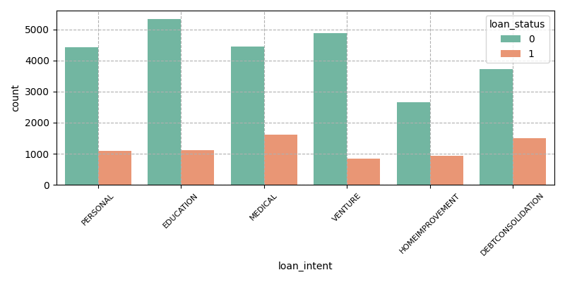
Figure 5: Loan intent

Y indicates that the borrower has defaulted before the loan, and N indicates that the borrower has no default record before the loan (Figure 6). Customers with past default records have relatively high credit risk, and financial institutions may have considered it when evaluating loans, and although they still grant loans, the possibility of them defaulting again is relatively high, so those with historical default records are relatively likely to default again. Customers with no past default record are generally considered to have a good credit profile, and financial institutions will give more trust when reviewing and lending, and at the same time, such customers may have relatively strong willingness and ability to repay, so most of them can maintain a non-default status.

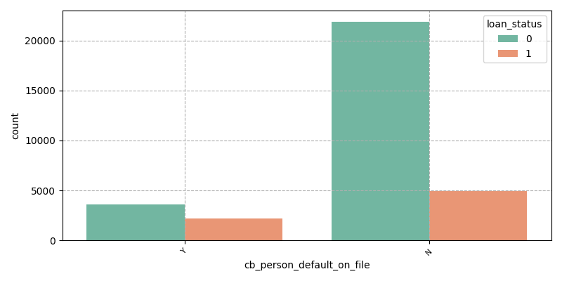
Figure 6: Historical default record

3.3. Continuous data analysis (corr>0.1 data)

Indicates that when the loan has a high percentage of income, it is more likely to default. Income and expenditure can be divided into several major parts, basic living expenses, health care expenses, entertainment expenses and debt repayment, when the loan amount accounts for a higher proportion of income, it is difficult for the borrower to repay, which can easily lead to default (Figure 7).

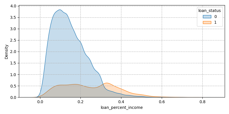
Figure 7: Loans as a percentage of income

Figure 8 shows that high interest rates will greatly increase the repayment cost of borrowers, and the default groups are relatively more distributed in the high interest rate range, peaking at 15% of the interest rate. They may be unable to afford high interest rates, and over time, the pressure to repay will increase dramatically, eventually leading to default.

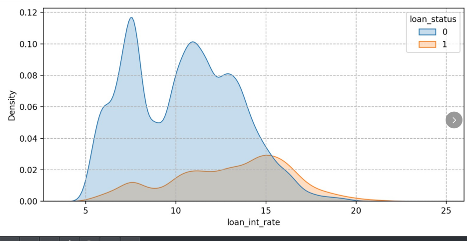
Figure 8: Loan interest rate

Large loans can be a heavy repayment burden. Defaulters may be overly optimistic about future income expectations and borrow more than they can afford, or the use of funds does not meet the expected returns, and eventually they are unable to repay, resulting in default (Figure 9)

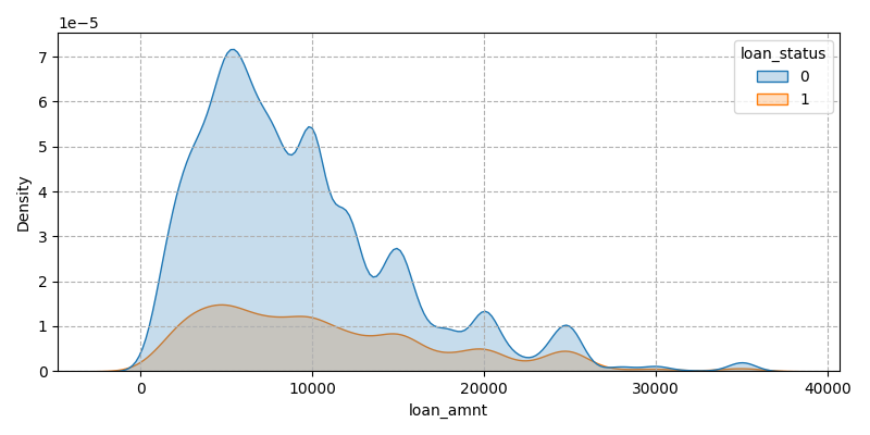
Figure 9: Number of loans

3.4. Model performance comparison

In terms of models, there are mainly tree model, logistic regression, CNN and DNN, CNN is suitable for capturing the correlation of spatial layout, DNN is suitable for unstructured data, and the data of the dataset in this paper is structured and needs to be strongly interpretive, so the tree model and logistic regression are the main experimental objects. In order to analyze which model performs better in credit default prediction, the performance of six models was compared through experiments, namely logistic regression, decision tree, random forest, GBDT, XGBoost and LightGBM. As can be seen from Figure 10, Figure 11 and Figure 12, XGBoost and LightGBM perform better overall, with AUC and Accuracy both above 0.925, and the recall and prcision of XGBoost and LightGB perform better on the six models in predicting whether a customer defaults.

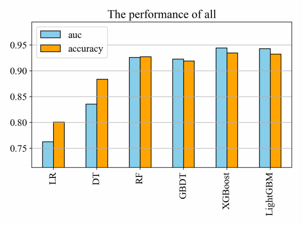
Figure 10: Overall performance of the experimental results

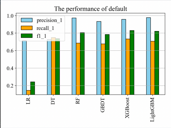
Figure 11: Predict the outcome of the defaulter experiment

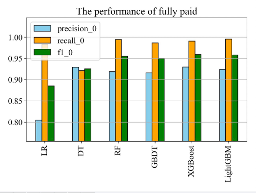
Figure 12: Predict the results of experiments on non-defaulters

3.5. Confusion evidentiary analysis

In order to further analyze which model has better performance, XGBoost or LightGBM, this part performs confusion evidence analysis. From Table 3, it can be seen that the precision=0.957 recall=0.733 of the XGBoost model and the precision=0.978 recall=0.707 of the LightGBM model before data balancing. After the data is balanced, the XGBoost model calculates precision=0.9124 recall=0.748 and the LightGBM model precision=0.914 recall=0.735. LightGBM performed better than XGBoost in terms of accuracy and XGBoost better than LightGBM in terms of recall, but the target variable was loan_status unbalanced (78% non-default vs. 22% default), so precision cannot be used as a basis for measuring the model (how many of all predicted non-default rates were actually non-default). Recall measures how many of the non-default categories are correctly identified as non-default. In order to predict credit risk users, this paper focuses on recall, so XGBoost was chosen as the prediction model, and the data is balanced on the dataset to improve the recall rate so that the majority of defaulters in the application process can be captured (Table 4).

Table 4: Evidence analysis of XGBoost and LightGBM confusion before and after data balancing

4. Discussion

After using SMOTE, the recall is significantly improved, mainly because SMOTE synthesizes new samples based on linear interpolation based on k-nearest neighbors in the feature space of minority samples, so that the positive and negative data in the dataset can be balanced, the identification ability of the model for minority classes is improved, and the missed detection is reduced, so as to improve the recall. While both XGBoost and LightGBM are gradient boosting trees, the basic idea of XGBoost is ensemble learning, where each model is specifically trained on the errors of the predecessor models, and these models are weighted together into a strong model. The regularization of XGBoost can suppress the complexity of the model and prevent overfitting. XGBoost can reduce the weight of some samples through regularization to avoid the model being misled, while LightGBM pays more attention to the training speed and has weak regularization ability. So XGBoost performs better in credit default forecasts.This paper verifies the effectiveness of SMOTE-XGBoost in credit default prediction, but there is still a lot of room for optimization in the face of the rapid development of fintech and the continuous upgrading of regulatory requirements. Future research can be explored in algorithms and scenario expansion. Technically, the current linear interpolation in SMOTE may not be able to capture the feature interaction relationship in the financial data set, so that the deeper relationship between the feature variable and the target variable cannot be mined. Subsequently, the implicit feature interaction can be carried out through DNN to improve the model's ability to capture complex risk patterns. In terms of scenario application, it can respond to the default of industry banks caused by economic fluctuations, establish industry characteristics association models, capture other data such as policy public opinion in real time, and accurately identify high-risk institutions.

5. Conclusion

In order to help financial institutions reject potential defaulting users, this paper uses SMOTE to deal with data imbalance and significantly improve the recall rate. In terms of model selection, the performance of six models was compared, and the performance of XGBoost and LightGBM was analyzed for confusion, and it was found that XGBoost had certain advantages, with an accuracy of 0.9124 and a recall rate of 0.748.This model can be applied to financial institutions with the goal of "potential defaulting users who refuse loans" to identify as many defaulting users as possible, reduce bad debt losses, and optimize the allocation of credit resources through higher recall rates.In the future, it is hoped that graph neural network (GNN) will be introduced to mine the hidden risk signals in unstructured data such as user social relationships. Explore the combination of automatic feature interaction generation (such as DeepFM) and dynamic weight adjustment to further improve the generalization ability of the model. At the same time, it is hoped that the effectiveness of the scheme will be verified on real datasets in the future.

References

[1]. LI Aihua,LIU Wanxin,CHEN Sifan & SHI Yong. Research on SMOTE-BO-XGBoost Integrated Credit Scoring Model for Unbalanced Data. Chinese Management Science, 1-10.doi:10.16381/j.cnki.issn1003-207x.2023.0635.
[2]. Khaoula Idbenjra, Kristof Coussement & Arno De Caigny. (2024). Investigating the beneficial impact of segmentation-based modelling for credit scoring. Decision Support Systems, 179, 114170-.
[3]. Zhang Qiong, Zhang Chang & (2025). Credit Risk Assessment of Commercial Bank Customers Based on Machine Learning. 365-374.
[4]. Mengyu Ren & Linghui Zhang. (2020). Research on Credit Risk Rating System of Bank of China. (eds.)
[5]. Shaoshu Li. (2024). Machine Learning in Credit Risk Forecasting — A Survey on Credit Risk Exposure.Accounting and Finance Research,13(2),
[6]. Xolani Dastile, Turgay Celik & Moshe Potsane. (2020). Statistical and machine learning models in credit scoring: A systematic literature survey. Applied Soft Computing Journal, 91, 106263-106263.
[7]. Belma Ozturkkal & Ranik Raaen Wahlstrøm. (2024). Explaining Mortgage Defaults Using SHAP and LASSO.Computational Economics,(prepublish),1-35.
[8]. LIU Manhu. (2023). Research on Credit Default Risk Prediction of a Commercial Bank Based on LightGBM (Master's Thesis, Chongqing University). Master https://link.cnki.net/doi/10.27670/d.cnki.gcqdu.2023.003390doi:10.27670/d.cnki.gcqdu.2023.003390.
[9]. Ruilin Hu & Tianyang Luo. (2023).XGBoost-LSTM for Feature Selection and Predictions for the S&P 500 Financial Sector.(eds.) Proceedings of the 2nd International Conference on Financial Technology and Business Analysis(part3)(pp.214-222). Rotman Commerce, University of Toronto;School of Management and Economics, Chinese University of Hongkong Shenzhen;
[10]. Kianeh Kandi & Antonio García Dopico. (2025). Enhancing Performance of Credit Card Model by Utilizing LSTM Networks and XGBoost Algorithms. Machine Learning and Knowledge Extraction, 7 (1), 20-20.
Cite this article
Chen,Z. (2025). Research and Analysis of Credit Default Prediction Based on Machine Learning. Advances in Economics, Management and Political Sciences,170,7-16.
Data availability
The datasets used and/or analyzed during the current study will be available from the authors upon reasonable request.
Disclaimer/Publisher's Note
The statements, opinions and data contained in all publications are solely those of the individual author(s) and contributor(s) and not of EWA Publishing and/or the editor(s). EWA Publishing and/or the editor(s) disclaim responsibility for any injury to people or property resulting from any ideas, methods, instructions or products referred to in the content.
About volume
Volume title: Proceedings of the 9th International Conference on Economic Management and Green Development
© 2024 by the author(s). Licensee EWA Publishing, Oxford, UK. This article is an open access article distributed under the terms and
conditions of the Creative Commons Attribution (CC BY) license. Authors who
publish this series agree to the following terms:
1. Authors retain copyright and grant the series right of first publication with the work simultaneously licensed under a Creative Commons
Attribution License that allows others to share the work with an acknowledgment of the work's authorship and initial publication in this
series.
2. Authors are able to enter into separate, additional contractual arrangements for the non-exclusive distribution of the series's published
version of the work (e.g., post it to an institutional repository or publish it in a book), with an acknowledgment of its initial
publication in this series.
3. Authors are permitted and encouraged to post their work online (e.g., in institutional repositories or on their website) prior to and
during the submission process, as it can lead to productive exchanges, as well as earlier and greater citation of published work (See
Open access policy for details).