1. Introduction

1.1. Background

For a long time, financial researchers have regarded stock markets as an important area of practical and theoretical research. With notable technical progress in recent years, such as big data and high-frequency trading, market data have grown substantially in terms of volumes. According to Kumar et al., it is challenging to analyze stock market trends, mainly due to factors like quarterly earnings announcements, noisy environments, and market news [1]. Traditional statistical methods and linear models, such as GARCH and ARIMA, often fail to make accurate predictions when applied to deal with sequential financial data that are nonlinear and high-dimensional. As suggested by Shah et al., assumed stationarity, linearity, and normality rendered ARIMA and GARCH, among other traditional models, less effective when used to model the non-linear and volatile stock market data [2].

In recent years, deep neural networks (DNNs) have undergone significant advancements. Notably, fields like audio analysis, text processing and visual perception have seen great breakthroughs. Empowered by deep learning, layered models can automatically identify features across different degrees of complexity [3]. Yu and Yan suggest that deep learning algorithms construct deep neural networks (DNNs) with several invisible layers to process large-scale nonlinear data, so as to identify deeper patterns beyond the capabilities of traditional machine learning approaches [4]. As a result, academic focus has been given to how to apply deep learning methods to predict stock prices. The aim is to effectively identify complex changes and patterns in the financial markets.

It is of significant economic significance for various stallholders like individual investors, policymakers, fund managers and financial institutions, to accurately predict stock prices. To this end, research on DNNs-based stock prediction models offers both theoretical and practical implications. These tools can effectively mitigate financial risk and make investment decision-making more intelligent.

1.2. Related research

In the field of DNNs-based stock market prediction, much research has been conducted to analyze how to apply various forms of neural networks to make stock market prediction more accurate. Some representative research works are summarized as follows:

1.2.1. Stock market prediction based on deep neural networks

The objective of the hybrid model of LSTM and DNN architectures proposed by Alam et al. is to improve the accuracy and robustness of stock market predictions. The strengths of each component contribute to the mechanisms’ strong adaptability to different types of datasets and company profiles. The performance measure of MAE, MSE, R²and maximum error was used on model The findings show that the model is able to predict High accuracy and stable enough The hybrid model performed better than other neural networks and is a practical tool for making investment decisions in uncertain market conditions [5].

In another study, Yu and Yan put forward a forecasting framework that makes use of a DNN-enhanced LSTM model powered by phase space reconstruction (PSR) [4]. The techniques involve denoising, normalisation, and segmentation based on the time window, which enhance the quality of the input and the model structure. Subsequent fine-tuning involved selection of the best activation functions and training algorithms. The results of the experiment show that this method outperformed normal models like ARIMA, SVR, deep MLP and vanilla LSTM in four major metrics. Furthermore, it has also achieved high accuracy under many stock indices.

1.2.2. Stock market prediction based on Support Vector Machines (SVM)

The study of Rouf et al. focuses on preprocessing techniques, input data, and applied AI in literature review on stock market prediction (SMP) from 2011 to 2021. Furthermore, they find that support vector machines (SVMs) is the most frequently used model. Lastly, they observe DNNs and ANNs make more accurate predictions with much greater efficiency. In addition, predictive performance could be enhanced through the integration of market data and online textual information. The study demonstrated the main obstacles to accurate prediction and issues that remained to be solved in the context of SMP systems [6].

1.2.3. Systematic review of stock market prediction

Kumar et al. reviewed 30 survey studies conducted on mathematical and machine learning methods in the context of predicting stock prices. Mathematical and machine learning techniques fall under different categories based on their methodology. Some research combined various methods in order to make more accurate predictions. Successful cases included the combination of ANNs and neural networks (NNs). Some of the hybrid models have been used in practice to predict and monitor stock market fluctuations and trends. It should be noted that using only historical data, existing techniques cannot make accurate stock price predictions, mainly due to consumer sentiment and government policies, among other factors external factors. Therefore, future research should analyze how to make the predictive models more reliable [1].

1.3. Objective

The study analyzes two representative deep learning models, namely LSTM and MLP models, in terms of their capability to identify predictive patterns from historical stock data, facilitating stock market prediction. It aims to make accurate stock price predictions by utilizing the respective advantages of both models in capturing meaningful patterns from a substantial amount of historical stock data. This research overcomes the limitations of traditional technical and statistical methods in processing time-dependent market data that are nonlinear and high-dimensional. As such, it aims to help make more reliable stock price predictions. In addition, it also seeks to help make investment decision-making more intelligent and data-based and mitigate financial risks for individual investors.

Following the goals of the research, this paper compares LSTM and MLP during periods of high and low volatility, high-price and low-price periods, as well as during the use of large dataset and small dataset. In different contexts, this study assesses the performance of both models, demonstrating the performance of the deep learning method in financial forecasting. As such, the findings of this study provide practical and empirical implications for future research aimed at improving stock price prediction strategies.

2. Method and data

2.1. Model architecture

To achieve these goals, LSTM and MLP model comparisons are systematically performed under the requirements of the high price period and low price period, high volatility period and low volatility period, small data set and large data set market conditions. The study showcases the performance of models and how the deep learning techniques behave during the forecast in the finance field. It offers useful information and evidence for enhancing future prediction models.

2.2. Model architecture

Two kinds of deep learning models—Multi-Layer Perceptron (MLP) and Long Short-Term Memory (LSTM) networks—are utilized in this work to forecast stock prices. Because of their great skill in capturing nonlinear patterns in data, both models are commonly used for time series prediction tasks.

2.2.1. Multi-Layer Perceptron (MLP)

Neural networks structures used in deep learning are called multi-layer perceptrons (MLPs) or deep feedforward networks [7]. A typical MLP consists of one or more hidden layers and one output layer. Each neuron in the layer is entirely linked to every other neuron in the layer. The network encompasses weighted sums and nonlinear activation functions and more on its input features, allowing the model to learn the relationships between input variables and target output. MLP's mathematical expression for forward propagation is described below:

\( {z^{l }}={W^{l}}{a^{l-1}}+{b^{l}} \) (1)

\( {a^{l}}=σ({z^{l}}) \) (2)

In the above two formulas, \( {W^{l}} \) and \( {b^{l}} \) represent the weight matrix and bias vector for the l-th layer. The term \( {a^{l-1}} \) denotes the output from the previous layer, or the input features when l = 1. The activation output of layer l is given by \( {a^{l}} \) , where \( σ \) denotes a nonlinear activation function such as ReLU, Sigmoid, or Tanh.

Using backpropagation in combination with gradient-based optimization methods like stochastic gradient descent (SGD) or Adam, MLPs are trained by minimizing an appropriate loss function. For SGD, model parameters are changed iteratively according to the following update rules:

\( {W^{l }}← {W^{l}}- η\frac{∂L}{∂{W^{l}}} \) (3)

\( {b^{l}} ← {b^{l}}- η\frac{∂L}{∂{b^{l}}} \) (4)

Here, \( {W^{l }} \) and \( {b^{l}} \) are the weight matrix and bias vector for the l-th layer; L is the loss function used to measure prediction error; and η is the learning rate that sets the step size during parameter updates. The network progressively lowers the loss function by means of forward and backward propagation, hence improving its capacity to generalize to unobserved inputs.

2.2.2. Long Short-Term Memory (LSTM)

The instability of the gradient during the training results in Standard Recurrent Neural Networks often having trouble with the long-range dependency [8]. To resolve this issue, Hochreiter and Schmidhuber proposed Long Short-Term Memory (LSTM) networks, a type of RNN that can keep information for long periods of time [9]. LSTM Network is a novel architecture Constant Error Carousel(CEC) which enable the constant error as the output to backpropogate through the special memory cells. In addition, the input, output, forget gate units have been employed for the controlling flow of information to and from the memory cells thus enabling the model to keep or omit information during every time step [8]. With this feature, the LSTM network can learn dependencies across sequences over 1000 time steps. This allows for complex modelling and long range patterns. The LSTM architecture consists of many essential functions that have specific mathematical equations. First, the forget gate is defined as follows:

\( {f_{t}}=σ({W_{f}} ·[{h_{t-1}},{X_{t}}]+{b_{f}}\ \ \ \) (5)

The input gate then regulates the inclusion of new data into the memory cell, modifying or overwriting the previous state. This is computed as follows:

\( {i_{t}}=σ({W_{i}} ·[{h_{t-1}},{X_{t}}]+{b_{i}}\ \ \ \) (6)

\( {C_{t}}=tanh({W_{c}}·[{h_{t-1}},{X_{t}}]+{b_{c}}\ \ \ \) (7)

Multiply \( {i_{t}} \) by \( {C_{t}} \) , and then add the forget gate information to obtain the new \( { C_{t}} \) . The expression is

\( {C_{t}}={f_{t}}×{C_{t-1}}+{i_{t}}×{C_{t}}\ \ \ \) (8)

To produce the hidden output, the output gate combines the present memory state \( { C_{t}} \) , the prior hidden activation \( { h_{t-1}} \) , and the input at time step t, \( {X_{t}} \) . The computation is given as:

\( {o_{t}}=σ({W_{o}} ·[{h_{t-1}},{X_{t}}]+{b_{0}}\ \ \ \) (9)

By processing the current input \( {X_{t}} \) and the prior hidden state \( { h_{t-1}} \) , the forget gate \( {f_{t}} \) evaluates and filters out irrelevant components of past information. Its output lies in the range [0,1], regulated by the sigmoid function. The tanh function is used to scale the candidate values to the range [−1, 1], ensuring stability in learning [10]. In this study, the LSTM model is employed for stock price prediction (see Figure 1).

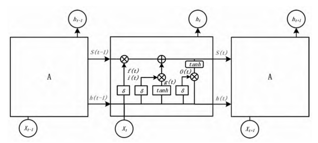
Figure 1: Unit structure diagram of LSTM neural network

2.3. Data

This study utilizes two datasets to assess the performance of deep learning models under varying data conditions. The main dataset comprises historical daily stock prices of Google (ticker symbol: GOOG), retrieved from Yahoo Finance. Spanning from August 19, 2004, to December 5, 2023, it includes a total of 4,858 entries. The detailed structure of the dataset is presented in Table 1.

Table 1: Data structure of Google Stock Price Dataset

Table 2: Data structure of World Stock Price Dataset

In addition to the Google dataset, a secondary dataset — the World Stock Prices Dataset — was employed to perform comparative experiments on a larger dataset. This dataset covers stock market data from multiple companies across different industries and countries between January 3, 2000, and February 28, 2025, totaling 304,180 records. The detailed structure is presented in Table 2.

While the primary analysis focuses on Google’s stock data, the World dataset was used to examine how the model performances change when trained and tested on a substantially larger and more diverse dataset.

In this study, data preprocessing involved several key steps to prepare the two stock price datasets for modeling. The “Date” field was standardized to datetime format, and the data were chronologically sorted; for the World Stock Price dataset, sorting was performed by both “Ticker” and “Date” to account for multiple companies. A five-day sliding window was applied to the features to generate lagged variables, which were then concatenated to form the input matrix. The next day’s closing price was set as the prediction target. After removing rows with missing values introduced by the shifting process, the dataset was partitioned into training and testing portions, with 80% used for training and 20% reserved for evaluation, preserving temporal order to avoid information leakage. Standardization was applied to both features and targets, and for the LSTM model, the input matrices were reshaped into three-dimensional arrays (samples, time steps, features) to meet sequential modeling requirements. This preprocessing pipeline ensured clean, normalized, and temporally structured data, thereby enhancing model training efficiency and predictive accuracy.

2.4. Experimental setup

In this study, both the LSTM and MLP models were implemented and fine-tuned for performance comparison under multiple conditions. The experiments were conducted using the preprocessed Google stock dataset as the primary source, and the World Stock Prices dataset as an auxiliary large-scale dataset for validation.

The implemented LSTM architecture includes two stacked LSTM layers: the first layer contains 64 units and is set to return sequences, while the second layer comprises 32 units. Following these, a fully connected dense layer with 32 neurons and ReLU activation is added prior to the output layer. The model is trained using the Adam optimizer and optimizes the Mean Squared Error (MSE) loss function. ReLU is adopted as the activation function in all hidden layers. For training, the model is run for 100 epochs on the Google dataset and 20 epochs when applied to the larger World Stock Prices dataset.

The MLP model uses the MLPRegressor from the scikit-learn library. The architecture includes two hidden layers with 50 and 80 units respectively. The model uses default ReLU activations and is trained using backpropagation with a maximum of 500 iterations. A fixed random seed (42) was set to ensure reproducibility.

3. Results

The experiment involved comparing the performance of LSTM and MLP models across several different market scenarios, including high and low price ranges, high and low volatility periods, and small versus large datasets. In this study, high-price and low-price periods were defined by using the median value of the “Close” prices as the threshold: records with a closing price above the median were classified as high-price, while those below or equal to the median were classified as low-price. Similarly, volatility was measured by the difference between the daily “High” and “Low” prices, and the median volatility value was used as the threshold to separate high-volatility and low-volatility periods. These partitioning strategies were applied to the Google stock price dataset to ensure a consistent and data-driven evaluation of model performance under different market conditions.

3.1. High price range

In high-price periods, both LSTM and MLP models performed similarly. LSTM slightly outperformed MLP in terms of MAE and RMSE, but the difference in R² was negligible, indicating both models are effective under such market conditions, as shown Table 3. Figure 2 shows that the prediction errors of both models are centered around zero, with the LSTM displaying a slightly narrower spread, indicating more consistent predictions. As illustrated in Figure 3, both models’ predicted values align closely with the ideal fit line, with LSTM results exhibiting slightly less dispersion, further confirming its marginal advantage.

Table 3: Result comparison in high price range

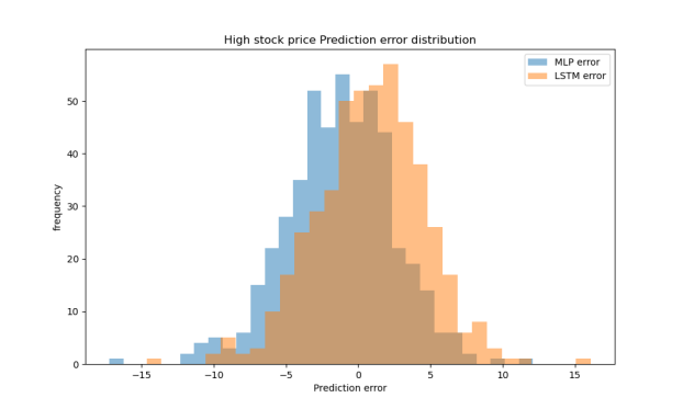
Figure 2: The distribution of prediction errors in the high price range

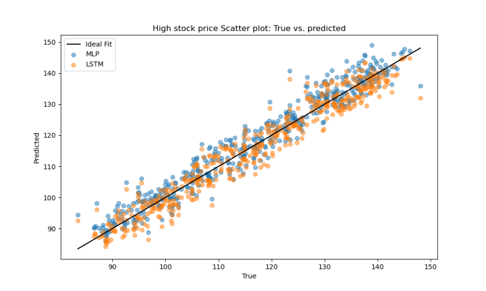
Figure 3: Scatter plot of the prediction results in the high price range

3.2. Low price range

In low-price scenarios, the MLP model clearly outperformed LSTM, particularly in MAE and R². The LSTM model showed significantly lower R² values, indicating weaker fitting performance when prices are low (Table 4). Figure 4 shows that the MLP model’s prediction errors are more tightly clustered around zero, indicating greater stability, while the LSTM errors are broader and more dispersed. As shown in Figure 5, MLP predictions align closely with the ideal fit line, whereas LSTM predictions exhibit systematic underestimation, further supporting MLP’s superior performance in low-price scenarios.

Table 4: Result comparison in low price range

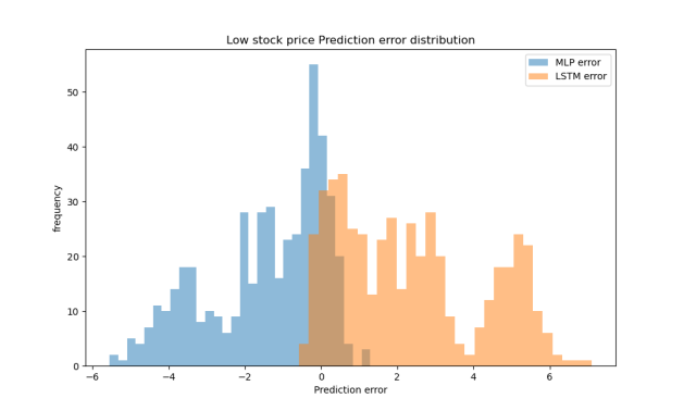
Figure 4: The distribution of prediction errors in the low price range

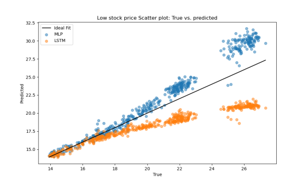
Figure 5: Scatter plot of the prediction results in the low price range

3.3. High volatility

Under high volatility, both models achieved decent prediction accuracy. LSTM had slightly worse MAE and MSE than MLP, but overall, both models demonstrated stable predictive power in this context (Table 5). Figure 6 shows that the prediction errors of both models are approximately symmetric and centered around zero, indicating a generally unbiased prediction tendency. In Figure 7, both models’ predicted values closely follow the ideal fit line, with minor scattering, further confirming the robustness of their performance under volatile market conditions.

Table 5: Result comparison in high volatility range

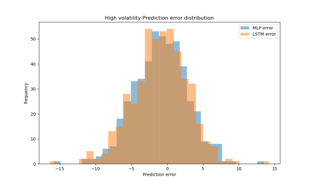
Figure 6: The distribution of prediction errors in the high volatility range

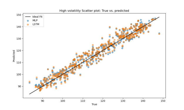
Figure 7: Scatter plot of the prediction results in the high volatility range

3.4. Low volatility

LSTM showed significant advantages in low-volatility conditions. It achieved much lower MAE and MSE compared to MLP, and higher R², indicating a stronger ability to capture smooth, stable market trends (Table 6). As shown in Figure 8, the LSTM model’s prediction errors are more concentrated around zero, while MLP errors are more widely spread, suggesting greater stability for LSTM. In Figure 9, LSTM predictions align more closely with the ideal fit line, whereas MLP results show greater deviation, further confirming LSTM’s superior performance in low-volatility scenarios.

Table 6: Result comparison in low volatility range

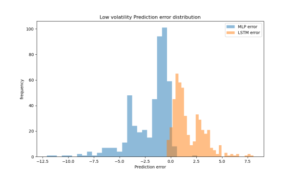
Figure 8: The distribution of prediction errors in the low volatility range

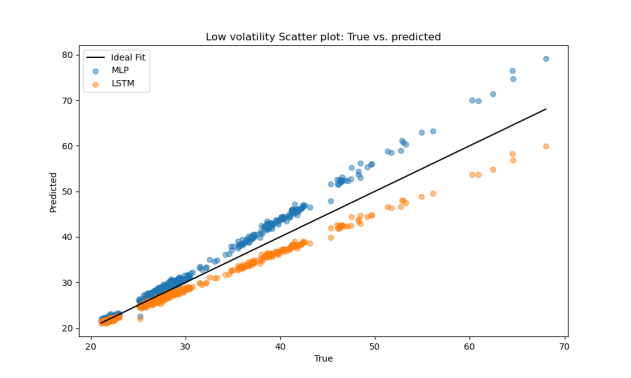
Figure 9: Scatter plot of the prediction results in the low volatility range

3.5. Small dataset (Google)

On the small Google dataset, MLP consistently outperformed LSTM across all metrics. The results (Table 7) suggest that MLP has a stronger capacity to learn from limited data without overfitting, while LSTM requires more training data to perform effectively. As shown in Figure 10, MLP’s prediction errors are more narrowly concentrated around zero, whereas LSTM exhibits a wider spread, indicating greater instability. In Figure 11, MLP predictions closely follow the ideal fit line, while LSTM predictions show a systematic underestimation, further confirming MLP’s superior performance on small datasets .

Table 7: Result comparison in small dataset

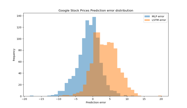
Figure 10: The distribution of prediction errors in small dataset

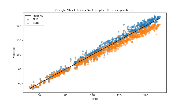
Figure 11: Scatter plot of the prediction results in the small dataset

3.6. Large dataset (World)

On the large-scale World Stock Prices dataset, both models demonstrated strong predictive performance. As shown in Table 8, their MAE, MSE, RMSE, and R² values were all very close, indicating high accuracy and stable fitting ability. Figure 12 shows that the prediction errors of both models are tightly concentrated around zero, with only minor dispersion. In Figure 13, the predicted curves of MLP and LSTM both closely follow the true value curve, accurately capturing the general trend and fluctuations in stock prices. These results confirm that both MLP and LSTM are effective for large-scale stock price prediction tasks.

Table 8: Result comparison in large dataset

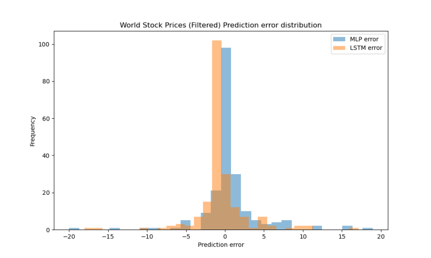
Figure 12: The distribution of prediction errors in large dataset

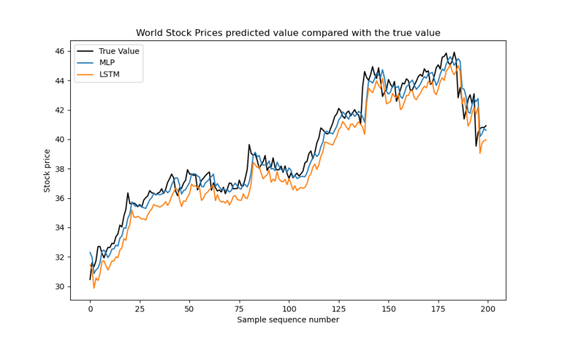
Figure 13: Comparison of predicted and actual values

4. Conclusion

Stock price forecasting remains a central topic and a persistent challenge in financial research. With the rise of big data, deep learning models have emerged as effective tools for improving prediction accuracy. Reliable forecasts can support decision-making for investors, fund managers, and financial institutions, contributing to better returns and lower financial risks.

The study assessed the forecasting capabilities of two commonly adopted deep learning models: MLP and LSTM, across various market scenarios. Through systematic experiments on both the Google stock dataset and the World Stock Prices dataset, the research evaluated model performance under high-price, low-price, high-volatility, low-volatility, small-scale, and large-scale data conditions.

The results demonstrate that both MLP and LSTM models are capable of achieving high prediction accuracy. In particular, LSTM exhibited notable advantages in capturing smooth trends during low-volatility periods, while MLP showed better robustness on smaller datasets with limited training samples. In large-scale datasets, both models performed comparably, indicating their effectiveness in modeling complex financial time series data.

The observed differences in model performance can be attributed to several factors. First, due to the relatively straightforward feature set (mainly information on price and volume), the LSTM model may have become less capable to give full play to its sequence modeling advantages, since richer, multi-dimensional temporal features are an important condition for the excellent functioning of LSTM. Second, LSTM may have been more vulnerable to the issue of overfitting Because the Google dataset is relatively small compared to the complexity of the LSTM model, while MLP shows better generalizability since its structures are simpler. In contrast, when data is large-scale and smoother, LSTM becomes more effective in capturing long-range temporal differences.

In summary, this study makes a detailed comparative analysis of various deep learning models in terms of their advantages and limitations when used to predict stock prices. When applied to capture long-term differences and similar trends, LSTM networks are more capable, By contrast, MLP models, due to simpler designs, proved to be more competitive when there is limited data available. This study, based on empirical analysis, demonstrates that under the condition of proper structure and application, deep learning models can effectively predict stock prices and make investment decision-making more intelligent. Future research could integrate several models to improve the accuracy of prediction, combine supplementary inputs, including media sentiment and economic variables, and develop models adaptable to the dynamic changes in the volatile stock markets.

References

[1]. Kumar, D., Sarangi, P.K., and Verma, R. (2022) A systematic review of stock market prediction using machine learning and statistical techniques. Materials Today: Proceedings, 49, 3187–3191.
[2]. Shah, D., Isah, H., and Zulkernine, F. (2019) Stock Market Analysis: A Review and Taxonomy of Prediction Techniques. International Journal of Financial Studies, 7(2), 26.
[3]. LeCun, Y., Bengio, Y., & Hinton, G. (2015). Deep learning. nature, 521(7553), 436-444.
[4]. Yu, P., and Yan, X. (2019). Stock price prediction based on deep neural networks. Neural Computing and Applications, 32(5), 1609–1628.
[5]. K. Alam, M. H. Bhuiyan, I. U. Haque, M. F. Monir, and T. Ahmed, “Enhancing Stock Market Prediction: A Robust LSTM-DNN Model Analysis on 26 Real-Life Datasets,” IEEE Access, vol. 12, pp. 122757–122768, Sep. 2024,
[6]. Rouf, N., Malik, M. B., Arif, T., Sharma, S., Singh, S., Aich, S., & Kim, H.-C. (2021). Stock Market Prediction Using Machine Learning Techniques: A Decade Survey on Methodologies, Recent Developments, and Future Directions. Electronics, 10(21), 2717.
[7]. Goodfellow, I., Bengio, Y., Courville, A., & Bengio, Y. (2016). Deep learning (Vol. 1, No. 2). Cambridge: MIT press.
[8]. R. C. Staudemeyer and E. Rothstein Morris, Understanding Long Short-Term Memory Recurrent Neural Networks – a tutorial-like introduction, arXiv preprint arXiv:1909.09586, 2019. Available: https://arxiv.org/abs/1909.09586
[9]. S. Hochreiter and J. Schmidhuber, "Long Short-Term Memory," in Neural Computation, vol. 9, no. 8, pp. 1735-1780, 15 Nov. 1997.
[10]. Jiang Shuyu. (2025). Stock Price Prediction Based on LSTM Model. Jiangsu Business Theory (01), 83-86.
Cite this article
Duan,Y. (2025). Stock Price Prediction Using Deep Neural Networks: A Comparative Study Between MLP and LSTM. Advances in Economics, Management and Political Sciences,193,1-13.
Data availability
The datasets used and/or analyzed during the current study will be available from the authors upon reasonable request.
Disclaimer/Publisher's Note
The statements, opinions and data contained in all publications are solely those of the individual author(s) and contributor(s) and not of EWA Publishing and/or the editor(s). EWA Publishing and/or the editor(s) disclaim responsibility for any injury to people or property resulting from any ideas, methods, instructions or products referred to in the content.
About volume
Volume title: Proceedings of ICEMGD 2025 Symposium: Innovating in Management and Economic Development
© 2024 by the author(s). Licensee EWA Publishing, Oxford, UK. This article is an open access article distributed under the terms and
conditions of the Creative Commons Attribution (CC BY) license. Authors who
publish this series agree to the following terms:
1. Authors retain copyright and grant the series right of first publication with the work simultaneously licensed under a Creative Commons
Attribution License that allows others to share the work with an acknowledgment of the work's authorship and initial publication in this
series.
2. Authors are able to enter into separate, additional contractual arrangements for the non-exclusive distribution of the series's published
version of the work (e.g., post it to an institutional repository or publish it in a book), with an acknowledgment of its initial
publication in this series.
3. Authors are permitted and encouraged to post their work online (e.g., in institutional repositories or on their website) prior to and
during the submission process, as it can lead to productive exchanges, as well as earlier and greater citation of published work (See
Open access policy for details).