1. Introduction

The financial industry is now maturing, and people are trying to get into the stock market to make more profits. Meanwhile, economic globalization has become an inevitable trend, with increasing economic exchanges between countries. The price trends of stocks serve as an important tool for measuring the level of market development. Therefore, adopting appropriate methods to study stock prices carries significant importance. Stocks encompass various factors such as opening price, closing price, highest price, and lowest price, among others. By focusing on these aspects to conduct research, fitting suitable models for stock price prediction can more effectively grasp the trends in stock prices. Since the development of the virtual economy, people have employed different approaches and perspectives to study the stock market. Since the inception of this industry, considerable achievements have already been made.

Since Covid-19, the economic recession has been serious. Ansari Saleh Ahmar in his paper indicated that Covid-19 made the whole world lockdown, it made a serious economic impact worse than economic decline [1]. People know the stock market is a important part of economics. Aravind Ganesan pointed out in his research, stock markets not only related to economic factors, but it also related to rational, social and other factors [2].

Banhi Guha pointed out that investors want to minimize the risk. So the most efficient way to minimize the risk is to use mathematical models to predict stock trends [3].

Ansari compared ARIMA, SutteARIMA and Holt – Winters methods to determine the most efficient model to predict stock market trends [1].

In Aravind Ganesan ' s research, he pointed out the ARIMA Model guarantees accuracy in a short period of time [2].

Setyo Tri Wahyudi once mentioned that he chose ARIMA Model to forecast stock market because of simplicity and wide acceptability. In order to forecast stock trends, velocity is a important aspect, because stock market might be changed in short [4].

In order to use ARIMA model to predict stock price , need data of past years.

Bharat Kumar Meher obtains observations from 2017 to 2019 , aims to build the ARIMA model and ensure its accuracy mostly [5].

Setyo Tri Wahyudi obtains Indonesia sample from 2010 to 2014 . Especially, he found that using ARIMA model to predict stock market has potential in tech . With tech ’ s development , using ARIMA model could become more accurate and more effective predictably [4].

Khan and Alghulaiakh's research, published in the International Journal of Advanced Computer Science and Applications, investigated the efficacy of the Autoregressive Integrated Moving Average (ARIMA) model for achieving accurate forecasts in stock market time series data. Their findings underscore the model's capacity to capture temporal autocorrelations inherent in stock prices, thereby demonstrating its utility for investors and financial analysts engaged in predictive modeling of market trends [6].

Dhyani et al. explored the application of the ARIMA model as a technique for stock market forecasting in their research published in the International Journal of Recent Technology and Engineering. Their work contributes to the understanding of how ARIMA can be utilized to analyze historical stock data and generate predictions regarding future price movements. This study provides insights into the practical implementation and potential of the ARIMA methodology within the financial domain [7].

Mondal examines the ARIMA model's effectiveness in predicting stock prices for fifty-six Indian stocks across various sectors. It investigates how different historical data periods influence prediction accuracy, employing the AIC for model comparison. Key contributions include a broad analysis of Indian stocks, sector-specific evaluations, and an assessment of the impact of historical data length on forecast precision [8].

Predicting stock market trends using the Autoregressive Integrated Moving Average (ARIMA) model necessitates the utilization of historical stock data spanning several years. Subsequently, the model's parameters are optimized through the application of information criteria such as the Akaike Information Criterion (AIC) and the Bayesian Information Criterion (BIC). To gain a deeper understanding of the impact of stock price fluctuations on the broader economy, an ARIMA model was developed to analyze the historical trends in JPMorgan Chase's stock prices. Obviously, try utilizing ARIMA model to predict stock market need data of past years. Then, optimize model parameters with AIC and BIC metrics.In order to better understand the impact of stock price fluctuations on the economy, an ARIMA model was established to study the trends of JPMorgan Chase stock prices.

2. Data & methodology

This study is based on partial daily data which are obtained from Investing. And collected data of JPMorgan (Ticker JPM) ranging from April 2022 to April 2025. It included date, open, closing, high, low, trading volume and rise &fall amount. This paper aims to predict stock trends, analysts determine building ARIMA model. ARIMA (Auto Regressive Integrated Moving Averge) model, as shown in Table 1.

Table 1: Past data of JPMorgan

2.1. Component of ARIMA

ARIMA model’ s effectiveness based on several core part, include AR, Differencing, and MA .

2.1.1. Part 1: AR

AR models build predictions rely on the past values of the variables themselves.

\( {Y_{t}}=c+\sum _{i=1}^{t} φi{Y_{k-i}}+{ξ_{t( \prime )}} \) (1)

2.1.2. Part 2: differencing

Differencing is a step in the preprocessing of time-series data, aimed at transforming a non – stationary time series into a stationary one. Difference is a mathematical operation that calculates the difference between adjacent data points in a set of numerical sequences. In the case where the sequence is still not stationary after the first-order difference. Nth-order differentials are required to make the sequence smooth.

\( Δ{Y_{t}}={Y_{t}}+{Y_{t-1}} \) (2)

2.1.3. Part 3: MR

The MA model takes into account the correlation of residuals in the time series, i.e., the historical value of the error term is combined in the model.

\( {Y_{t}}=μ+{ε_{t}}+\sum _{i=1}^{t} {\overline{θ}_{i}}{ε_{t-I}} \) (3)

2.2. Formula of ARIMA

Total ARIMA model formula:

\( c+\sum _{i=1}^{t} {φ_{i}}{Y_{k-I}}++\sum _{i=1}^{t} {θ_{i}}{ε_{t-I}}+{ε_{t}} \) (4)

Y_t : Time series data being considered

φ_i : The parameters of the AR model, which are used to describe the relationship between the current value and the value of the last p time points

θ_i : The parameters of the MA model, which are used to describe the relationship between the errors of the current value at the last q time points

ε_t: Error term at time t

c : Constant terms

The ARIMA model is based on the combination of these three components to accurately describe the statistical properties of a time series through model parameters. Practically , we need to calculate the p (The order of the autoregressive term) , d (Differential order) and q (The order of the moving average item) . Determining these parameters is a critical step in prediction, p , d and q have a direct impact on the predictive power of the model.

2.3. Data preprocession

In Time-series analysis, data preprocession is the most important step. Data preprocessing includes three main parts: data cleaning technology, data smoothing processing, and data normalization and standardization.

Initially, a rigorous data cleansing procedure was undertaken to identify and rectify errors and inconsistencies, thereby ensuring the integrity of the dataset. During the subsequent model development phase, the presence of missing values necessitated the implementation of appropriate imputation techniques. Specifically, missing data points were addressed by employing a value imputation strategy. Potential imputation methods considered included the substitution of missing values with the mean, median, or mode of the respective variable, with the final selection based on the distributional characteristics of the data. Furthermore, the dataset was examined for the presence of outliers, defined as observations exhibiting significant deviations from the central tendency. To manage these extreme values, both statistical and model-based approaches were considered for their detection and potential handling.

2.4. Data smoothing processing

Differential is one of the common methods for smoothing time series data. It usually divided into first-order difference and second-order difference. The other method is time series decomposition.

2.5. Data normalization and standardization

Data normalization and normalization are important steps in the preprocessing step. Adopt a normalization approach. Common methods such as min-max normalization linearly scale the data to the [0,1] interval. Another method is Z-score normalization, which is to convert the data into a distribution with a mean of 0 and a standard deviation of 1.

There are generally two ways to select ARIMA model parameters. Statistical methods for model ordering and Information Criterion Selection Method. Statistical methods for model ordering - ACF and PACF identification, In the ARIMA model, AR refers to the autoregressive term, and PACF can help invenctors determine this part of the parameters. MA refers to the moving average term, and ACF is used to determine this part of the parameter.

2.6. Train the model

The model fitting is the core step. It involves estimating model parameters using a training dataset. The parameters of the ARIMA model include: p, d, q. Steps to fitting the model included select parameters, build model, fitting dataset and perform the diagnostic tests. In ARIMA model training, it is very important to choose the appropriate parameters (p, d, q). This step is called model ordering. Grid search is a widely used method that finds the best set of parameters by systematically traversing all combinations of parameters within a specified range.

p : Autoregressive . Describes the lag values used in the model using observations.

The definition samw AR

q : Moving average. Describe the lag value used in the model to think about the error

The definition same as MA.

d : represents the order of the difference.

ARIMA Model Evaluation

After we build ARIMA model, it also to be evaluated. Two indicators were used for evaluation: MSE and MAE.

Mean Squared Error (MSE) is a common statistic used to measure the prediction error of a model.

The formula:

\( \sum _{i=1}^{n}(yi+ ỹi) \) (5)

Mean Absolute Error (MAE) is another metric commonly used to evaluate the performance of predictive models.

The formula:

\( \sum _{i=1}^{n}|yi- ỹ| \) (6)

N Represents the total number of data points.

3. Results

JPMorgan Chase's closing prices over the past three years are shown in Figure 1.

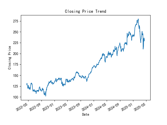
Figure 1: Closing price trend chart for JPM

Figure 2 indicated that from May 2022 to around the beginning of 2025, the closing price generally showed an upward trend. The price gradually climbed from a relatively low level at the beginning, reflrcting that the stock or financial asset as a whole is in an upward channel during this time. After the beginning of 2025, there is a clear downward trend in the price, breaking the previous upward pattern, perhaps the market environment has changed unfavorably for the asset, such as increased competition in the industry, unfavorable macroeconomic situation, negative events in the company itself, etc., which have changed the market's expectations for it, and the seller's power has increased, driving the price downward. Autocorrelation as shown in Figure 2.

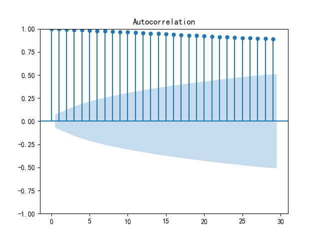
Figure 2: Autocorrelation for JPM

Figure 2 is Auto correlation Plot. In this graph, the height of each point in the graph represents the value of the autocorrelation coefficient corresponding to the lag order. As can be seen from the figure, the autocorrelation coefficient in the early period is close to 1 and remains high in the long lag order, indicating that the series has a strong correlation in a longer time interval.

Figure 3 is a Autocorrelation too, as you can see from the graph, the autocorrelation coefficient is 1 except when the lag order is 0. The autocorrelation coefficients of the other lag orders quickly fall into the random interval (in the gray area), indicating that the time series is stationary. In this graph, except for the high zero-order autocorrelation coefficient, the autocorrelation coefficient of other lag orders basically fluctuates around 0, indicating that the correlation of the series is weak in a long time interval, and the current value is mainly closely related to itself, and has little correlation with the value of the distant time point in the past.

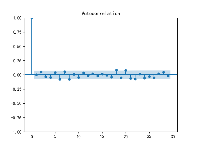
Figure 3: Autocorrelation plot (ACF)

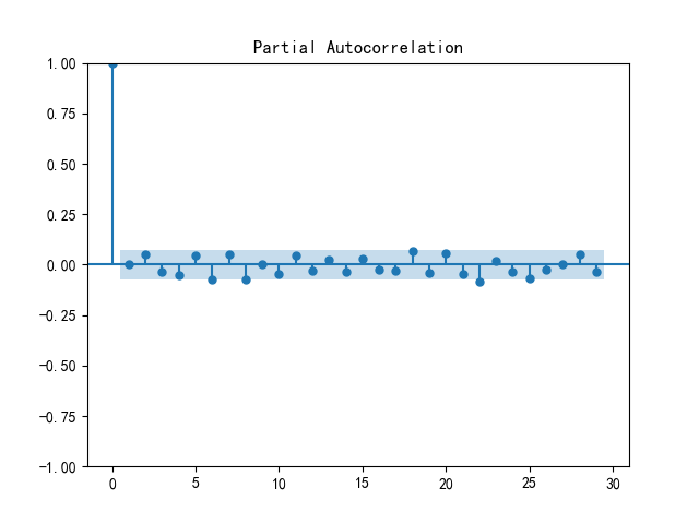
Figure 4: Partial autocorrelation(PACF)

Figure 4 is a Partial Autocorrelation plot. A partial autocorrelation plot can be used to assist in determining the p-value. In this graph, the partial autocorrelation coefficient quickly falls into the stochastic interval after a lag order of 1, indicating that the autoregressive order p may be 0 or 1 when building the ARIMA model. The graph shows that the partial autocorrelation coefficient of the lag order basically fluctuates around 0 except for the zero order, indicating that the direct correlation of the series on longer time intervals is weak, and there is no significant direct correlation between the current value and the value at a distant time point in the past.

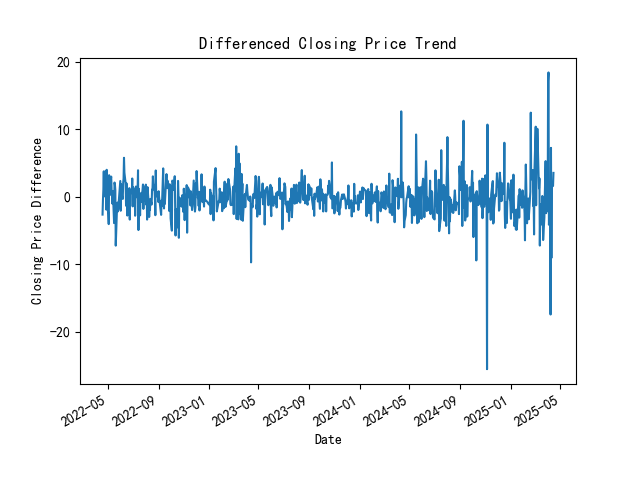
Figure 5: Closing price difference series trend chart

Figure 5 is Closing price difference series trend chart. The X-axis is the closing price difference and the Y-axis is the date. As can be seen from the figure, after the closing price is differential, the series fluctuates up and down around the zero value, and there is no obvious upward or downward trend, nor does it show periodic regular changes, indicating that the differential operation effectively eliminates the trend term in the original series. Conform to the characteristics of stationary time series. The figure shows the sequence after the first-order difference, which shows that when the original closing price series is analyzed, the series is smoothed by the first-order difference, so in the ARIMA model, the value of d is determined to be 1. Also, this differential series trend chart indicates that the series has leveled off.

Table 2: 5 Days results

In Table 2, the stock price forecast for the next 5 days, the column on the left is the mean, and the right is the floating range.

4. Discussion

The finalized model is ARIMA(0, 1, 0). In this model, the parameter “d = 1” shows that the original non - stationary time series has been turned into a stationary one through first - order differencing. The values of “p = 0” and “q = 0” imply that there is no autoregressive part and no moving average part. Basically, this model supposes that the next value is just the last observed value plus a random error term, which is a typical characteristic of a random - walk model. From this model, we can tell that the average price fluctuation range for the coming period isn't fixed at 179.85. Instead, it means the price will fluctuate randomly around this value. Besides what the random error shows, the model itself doesn't capture any inherent trend or pattern.

It's important to note that the data for this prediction model comes from JPMorgan. As a world - leading financial services firm, JPMorgan has professional expertise in data collection, processing, and model building. Its analysis usually depends on a large amount of historical data and strict financial reasoning. For example, JPMorgan's research on Boeing covers various aspects, like the company's revenue, profit, and its position in the industry. This provides a relatively solid data foundation for the model. But that doesn't mean the model is perfect. On January 29, 2025, JP Morgan kept its “overweight” rating on Boeing, with a latest target price of $200.00. This rating reflects JPMorgan's expectations for Boeing's long - term development. However, it's different from the prediction result of the current ARIMA(0, 1, 0) model, which shows the limitations of a single model.

In the financial market context, JPMorgan's model might focus too much on analyzing historical price series. It may overlook the immediate impact of specific events on stock prices. For example, events like the production increase of Boeing 737 MAX or winning the F - 47 contract in the defense business can affect the stock price. But the ARIMA(0, 1, 0) model, which only depends on historical price differences, can't include such influences. This shows the model's weakness in dealing with real - world complexities that can greatly change stock prices.

Looking at the final prediction results, it can see that the confidence interval has been widening since the first day. This indicates that the uncertainty is growing, which is in line with the characteristics of the random - walk model. As the prediction period gets longer, the cumulative effect of random fluctuations becomes more obvious, leading to larger model errors. A wide confidence interval means the model has less confidence in long - term predictions. For investors, although the model gives a central value (179.85), the actual price could be very different. This situation is also worth noticing in JPMorgan's analysis framework. The difference between its target price for Boeing and the current model prediction further shows that a single model can't accurately predict the stock price trend.

When making actual forecasts, we must consider the social situation and economic policies. JPMorgan's analysis also takes these macro - factors into account. For instance, changes in aviation safety regulations, fluctuations in the global economic growth rate, or adjustments to trade tariffs can all have a big impact on Boeing's stock price. Also, overall industry trends, such as the demand for new aircraft models or competition from other aerospace companies, are important. Moreover, company - specific events, like R & D breakthroughs, management changes, or legal issues, should be considered. By combining these factors - either by using advanced models that can include external variables (such as SARIMAX) or through comprehensive qualitative analysis - we can improve the accuracy and practical value of predictions. This comprehensive method ensures that predictions don't just rely on historical price patterns. Instead, they reflect the dynamic and complex nature of the real - world market environment, giving investors and analysts a better basis for decision - making.

In conclusion, JPMorgan's data and model offer an important angle for predicting Boeing's stock price. But the results of its ARIMA(0, 1, 0) model should be analyzed together with its overall rating and target price for Boeing, as well as other market factors. Only in this way can it comprehensively evaluates the future trend of Boeing's stock price.

5. Conclusion

In this paper, an ARIMA(0, 1, 0) time series model was employed to forecast stock prices. The model was established using historical stock price data, aiming to uncover patterns for prediction.

The analysis revealed that the prediction error of the ARIMA(0, 1, 0) model grew notably as the prediction period lengthened. For example, the confidence interval of the prediction expanded rapidly after the initial days, showing a high level of uncertainty in long - term forecasts. This was likely due to the model's simplicity. It couldn't fully consider complex market elements like sudden company - specific news or short - term market sentiment changes. Compared with more complex models in similar studies, this model had a relatively high error growth rate, demonstrating its limitations.

In real - world situations, stock prices are affected by numerous factors. Economic policies, such as interest rate adjustments and trade regulations, have a direct impact. For instance, an interest rate change can influence a company's cost of capital and profitability, thus affecting its stock price. Social conditions like public health events or political unrest also play a role. A public health event might disrupt a company's supply chain and lead to a stock price decline. However, the ARIMA(0, 1, 0) model used in this study didn't account for these external factors, contributing to the rising prediction error.

To enhance stock price prediction accuracy, future research is needed. With technological progress, more accurate models can be developed. Future studies could focus on integrating external variables like economic indicators and social sentiment data into time - series models. Machine - learning - based models, such as RNNs or LSTMs, are also promising. These models can better capture non - linear relationships in stock price movements, offering more reliable financial market analysis.

References

[1]. Ansari Saleh, A., Pawan Kumar, S., Nguyen Van, T., Nguyen Viet, T., & Vo Minh, H. (2022). Prediction of BRIC stock price using ARIMA, SutteARIMA, and holt-winters. Computers, Materials & Continua, 70(1).
[2]. Ganesan, A., & Kannan, A. (2021). Stock price prediction using ARIMA model. International Research Journal of Engineering and Technology (IRJET), 8(2395).
[3]. Guha, B., & Bandyopadhyay, G. (2016). Gold price forecasting using ARIMA model. Journal of Advanced Management Science, 4(2).
[4]. Wahyudi, S. T. (2017). The ARIMA Model for the Indonesia Stock Price. International Journal of Economics & Management, 11.
[5]. Meher, B. K., Hawaldar, I. T., Spulbar, C. M., & Birau, F. R. (2021). Forecasting stock market prices using mixed ARIMA model: A case study of Indian pharmaceutical companies. Investment Management and Financial Innovations, 18(1), 42-54.
[6]. Khan, S., & Alghulaiakh, H. (2020). ARIMA model for accurate time series stocks forecasting. International Journal of Advanced Computer Science and Applications, 11(7).
[7]. Dhyani, B., Kumar, M., Verma, P., & Jain, A. (2020). Stock market forecasting technique using arima model. International Journal of Recent Technology and Engineering, 8(6), 2694-2697.
[8]. Mondal, P., Shit, L., & Goswami, S. (2014). Study of effectiveness of time series modeling (ARIMA) in forecasting stock prices. International Journal of Computer Science, Engineering and Applications, 4(2), 13.
Cite this article
Peng,R. (2025). Using ARIMA Model Predict Stock Market. Advances in Economics, Management and Political Sciences,190,38-46.
Data availability
The datasets used and/or analyzed during the current study will be available from the authors upon reasonable request.
Disclaimer/Publisher's Note
The statements, opinions and data contained in all publications are solely those of the individual author(s) and contributor(s) and not of EWA Publishing and/or the editor(s). EWA Publishing and/or the editor(s) disclaim responsibility for any injury to people or property resulting from any ideas, methods, instructions or products referred to in the content.
About volume
Volume title: Proceedings of ICEMGD 2025 Symposium: Digital Transformation in Global Human Resource Management
© 2024 by the author(s). Licensee EWA Publishing, Oxford, UK. This article is an open access article distributed under the terms and
conditions of the Creative Commons Attribution (CC BY) license. Authors who
publish this series agree to the following terms:
1. Authors retain copyright and grant the series right of first publication with the work simultaneously licensed under a Creative Commons
Attribution License that allows others to share the work with an acknowledgment of the work's authorship and initial publication in this
series.
2. Authors are able to enter into separate, additional contractual arrangements for the non-exclusive distribution of the series's published
version of the work (e.g., post it to an institutional repository or publish it in a book), with an acknowledgment of its initial
publication in this series.
3. Authors are permitted and encouraged to post their work online (e.g., in institutional repositories or on their website) prior to and
during the submission process, as it can lead to productive exchanges, as well as earlier and greater citation of published work (See
Open access policy for details).