1. Introduction

Understanding the exchange rate (XR) and its determinants forms the fundamental crux of international economics through the purchasing power parity theory (PPP⁾, which is arguably one of the most surviving yet controversial frameworks. Based on the PPP theory, the exchange rates would equalize price levels across countries with a standard basket of goods in the presence of any transaction cost or any form of friction in the market. While this is conceptually simple and endowed ex-ante with intuitive appeal and face validity, it has been quite complex in empirical application, especially concerning economic diversity across countries. Countries’ currencies naturally have different purchasing powers due to variations in human capital, technological advancement, etc. Such a phenomenon was obvious during the fixed exchange rate era (where most countries had a stable exchange rate and foreign currency reserves) and even exaggerated in the following floating exchange rate era (where most countries decide fluctuation of their exchange rate is dependent on the foreign exchange market). The reasons that caused the different purchasing power of different economies cannot be associated unilaterally and are intricate in the nature of the economic system. Nevertheless, the exchange rate and its volatility are, still, undoubtedly, vital issues in international economics that impact heavily on global trade and investment and even economic stability. Moreover, exchange rate movements are unpredictable due to a complex interaction of influences because of macroeconomic variables, market sentiment, geopolitical events, and the reaction of governments. At this current time, the effects of these would most likely result in the very disruptive nature of the shocks in less-developed economies with weaker financial systems.

The study of exchange rates remains a cornerstone of international economics, with PPP theory providing one of the most enduring, yet contested, frameworks for understanding currency value dynamics. While PPP suggests that exchange rates should equalize price levels across countries by considering a basket of goods, the empirical reality has shown far more complexity due to variations in macroeconomic variables, technological advancement, and the heterogeneity of countries' economic systems. Added to this is the ever-volatile and unpredictable nature of the rate of exchange, which is influenced even more by geopolitical events, state-level interventions, and shifts in market sentiment, underlining again the need for nuanced exploration of this issue.

Although a considerable volume of research focused on the issues of exchange rate volatility-economic performance nexus, only a few have tried to present a strong long-run econometric analysis between real exchange rates and PPP and their impact on economic growth for both developed and developing economies. Existing literature, including that on currency undervaluation and its potential benefits for growth, often fails to address the institutional conditions that shape the success of such strategies, and they need to examine their long-term sustainability thoroughly.

This paper seeks to fill these critical gaps by utilizing advanced econometric techniques, including machine learning algorithms and OLS regressions, to rigorously test the long-term implications of real exchange rate undervaluation on economic growth across different levels of development. By analyzing a comprehensive dataset from the Penn World Table (PWT) Version 10.0, this study not only tests the validity of absolute and relative PPP but also aims to clarify whether certain countries benefit from maintaining an undervalued currency over extended periods. This work will offer policymakers key insights into exchange rate management, particularly in developing economies, where strategic currency undervaluation may also serve as a vital tool for fostering economic growth.

2. Literature review

A major implication of exchange rate volatility such as that is its tendency to have a depressing effect on productivity growth. More specifically, higher volatility suppresses productivity, making it more difficult for economies, especially those without a properly developed financial system, to achieve long-term economic growth [1]. Thus, in the face of so much uncertainty in such an environment, investors will abstain from investment, and efforts to attain any long-term economic planning will be non-committal. Advanced econometric models include the ARDL approach, which has been used to model both short- and exchange rate volatility’s long-run effects on productivity. It turns out that the bad influence of volatility is more pronounced for nations with less developed systems.

Moreover, the manipulation of currencies by the government aggravates the fluctuation in the exchange rate. Many governments have indeed contributed to this by devaluing their currencies to be competitive in international trade, making exports cheaper and more marketable. While such a strategy could turn out to be profitable in the short run, it contributed to the long-run instability of the world economic order. It is the manipulation of the currency that disrupts trade balances and may provoke corresponding responses from trading partners, ultimately amounting to what is called a currency war. Such practices further inflate the volatility of exchange rates, interfering with international markets and increasing the unpredictability of currency movements [2].

Different exchange rate regimes-fixed, floating, and manipulated-interact with monetary policy to produce varying degrees of stability or instability in economic performance. Econometric estimates better suggest that direct manipulation of policy-induced changes in exchange rates could be added to the inherently unpredictable variables of those exchange rates and make the task of economic management so much more complex than it would pose a formidable challenge to the nicety with which conventional models estimate economic behaviour [3]. The paper seeks to look into the real exchange rate (RER) in PPP measurement as well as its long-term impact on economic growth by testing whether certain countries benefit from an undervalued exchange rate.

Over the years, Purchasing Power Parity (PPP) has constituted a significant part of international economics, which reveals the theoretical base of how exchange rate configurations narrow down the variations in the price levels of goods across countries. Although initially suggested by Cassel back in 1918 as ‘an equilibrium exchange rate device within a framework of pure competition, free of transaction costs and barriers of trade’, PPP has been widely criticized, developed, and subsequently, a progressive investigation into its theoretical base and empirical application [4].

The significance of the change from fixed to floating regimes in the early 1970s marked part of the point in the direction that a new era of understanding showed toward PPP. In fixed exchange rate systems, PPP acted as the guide to the judgment of currency values. With the change to floating rates, the balance set new Citizen Kane forces in determining the value of a country's currency, while PPP simply died [5,6]. That change meant that more volatility and more flexibility crept into the system, and there had been more frequent and extraordinary deviations from the theoretical predictions of PPP.

That being said, the research question of this paper is considerably germane, especially for developing countries currently considering the undervaluation of their currency as a means to drive growth. This, in particular, would be the crucial question that still needs to be answered as it cuts across economic policy issues, global trade dynamics, and long-term development strategies. While existing pieces of literature, like Rodrik's research on RER and economic growth, underline the possible benefits of undervaluation of the currency for export competitiveness and structural transformation, deep analysis of the institutional contexts conditioning such strategies' success is often lacking [7]. Moreover, an in-depth discussion of their long-term sustainability and trade-offs—including inflation, debt accumulation, or financial instability—among others is not well presented in the corresponding grouping of countries based on development. Newly proposed theories, such as the Balassa-Samuelson effect, provide insights into how the RER deviates from PPP but do not cover how developing countries might use undervaluation effectively to drive growth. In addition, discussions on PPP and economic measurement are ahistorical and static, never getting to dynamic, policy-driven issues of RER management. In that respect, there has been a gaping hole in the literature on the subtle and long-run implications of RER undervaluation, particularly how this variable interacts with economic, institutional, and global factors. Hence, this paper aims to fill these gaps by utilizing a comprehensive analysis of the long-term implications of real exchange rate undervaluation via PPP on economic growth, particularly in the context of developing countries. It will explore the institutional factors, sustainability challenges, and global economic interactions that have been largely overlooked in the existing literature, offering a more nuanced understanding of whether and how certain countries might benefit from maintaining an undervalued currency as part of their growth strategy.

The effectiveness of PPP depends on many factors, such as how much a country has developed or the degree of openness to trade. For instance, economies with high mono-product dependency, i.e., OPEC, are certain to exhibit differences in their exchange-rate movement compared to a highly diversified economy. Moreover, even the openness of a country to international trade is likely to vary between the countries. This difference in market integration level further complicates the working of PPP. This paper explores the validity of the PPP model in different economies by comparing OPEC with others and applying the econometric approach.

Through the analysis of these distinct groups, it tries to explain how their structural differences impact the convergence of exchange rates toward relative price differentials, thereby offering key insights for policymakers when thinking about exchange rate management in diverse economic environments.

No less importantly, empirical work has emphasized the limitations of PPP. To give a particular example, the investigation of the long-term relationship between exchange rates and price levels went on with the cointegration theory, which is now more like Corbae and Ouliaris [4]. The results suggest strongly that, at least for the absolute version of PPP, it does not hold in the expected long-term equilibrium; this may be one reason for PPP having little applicability when dealing with non-stationary exchange rates. Rogoff has also referred to the "PPP puzzle," which states that real exchange rates do indeed revert to their PPP-implied values over the long run, but with considerable volatility in the short to medium-term and slow mean reversion [7]. A puzzle that strongly exemplifies how hard it is to use PPP for out-of-sample forecasts of exchange rate movements, especially considering other market frictions like transport costs and non-tradable goods.

Later, Sarno and Taylor delved deeper into the empirical evidence, and they still noted that PPP was an important benchmark inducer for long-term exchange rate analysis but noted various real-world aspects for its limited short-term predictive performance, like varied trade barriers and varied local consumption patterns [7]. All these results suggest the existence of widespread, persistent deviations of PPP behaviour across different economic settings. They also warrant an increased level of sophistication in the application of PPP, particularly in policymaking. This is underscored more in oil-exporting countries, having practical implications for PPP. The reason is obvious: in countries such as Iran, this relation of the price of oil to real exchange rates is significant. Jahan-Parvar and Mohammadi consider causality within the hypothesis of the Dutch Disease in the sense that an appreciation of oil prices creates an appreciation of RERee, unloading the non-oil sector, which becomes less competitive [8]. Consistency in finding such an effect is relevant in continually ensuring sustainable economic growth by managing the resource frontier and, as such, managing the exchange rates in resource-rich countries. Recent developments in econometric techniques have streamlined the tests conducted on PPP. For instance, Dupuis and Victoria-Feser have proposed a robust VIF regression method, which can improve measures by which outliers and multicollinearity problems related to large data sets are dealt with [9]. It allows putting more faith in empirical tests conducted for PPP. Hence, time and again, it provides more assured and reliable insight into the long-term relationship between the exchange rate and price levels [10]. Conclusion In conclusion, it can be said that PPP still forms the basic structure of international economics, but its empirical validity and practical application still need to be improved. In studying long-run exchange rate analysis, PPP can provide some helpful direction, but it has to be put about a general economic outlook. Future research can stimulate an accurate understanding of the features of PPP and its relations with the design of economic developments, considering the new global changes.

3. Data preparation

This paper used the data extracted from Penn World Table National Account Data version 10.0., which includes data on the productivity, income, input, output, and demographic information of 219 countries between 1950 and 2019.

3.1. Data cleaning

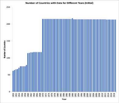
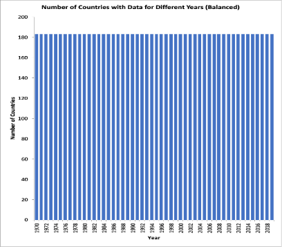
The first histogram in Figure 1 is generated to illustrate the distribution of data in the Penn World Table, listed by the number of countries with data in each year. Most countries have only had a complete data set since 1970 due to data availability. In order to keep a balanced panel for later uses, all data before 1970 is deleted. In addition, several countries also still need years of data from 1970 to 2019. Such include dissolved countries - the Soviet Union, Yugoslavia, Czechoslovakia, and Netherlands Antilles, as well as countries that have gained independence within the period, which as the Republic of Kosovo and Timer Leste. Since those planned economies are heavily influenced by strong government intervention, they need to be representative of the modern economic systems in this investigation. As a result, all of the countries stated above were also eliminated from the panel. Finally, 28 countries with missing GDP values from 1970-2019, such as post-Soviet states, as well as others, are eliminated in total. The data-cleaning process results in a balanced panel of data from 183 countries spanning 1970-2019, as shown by the second distribution in Figure 1.

3.2. Feature engineering

From the Penn World Table, values in Table 1 are extracted for our upcoming analysis. We use the same names for the variables as Penn World Table for simplicity.

All variables used in this paper are summarized in Table 2 and Table 3, grouped by the section they appear.

3.3. Data verification

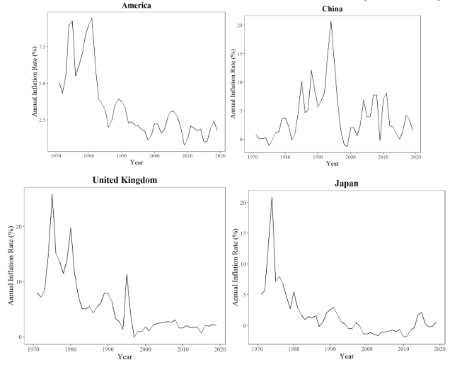
In order to test the authenticity of the dataset after processing, one method implemented is to generate line charts of the inflation rate of some familiar countries to check if the trends on these charts conform to the theoretical trends in the world (see Figure 2). According to the chart for China, the inflation rate around 1995 was significantly high. This phenomenon conforms to China’s reform and opening around the early 1990s, which expanded China’s consumer demand. Furthermore, the decline of Japan’s inflation rate exhibited on its chart corresponds to the deflationary pressure of the period called the “Lost Decade” in Japan after the 1980s, when the economic bubble of excessive asset prices collapsed. After the examination, the dataset is concluded to be ready for analysis.

4. The purchasing power parity theory

Generally, PPP theory suggests that the actual price levels in different currency systems approach the same over time, which indicates that different types of currencies are expected to have equal purchasing power for an identical basket of goods. In other words, after converting country A’s currency to country B’s, goods in country A should cost the same as goods in country B. In this money-converting process, the exchange rate is commonly used as a standard for trade. , to reflect the purchasing power of a certain currency, the price level ratio of the two countries must be incorporated into the calculation, which yields the Real Exchange Rate. Here, the RXR of the country’s currency is calculated against US dollars since the exchange rate in the Penn World Table is measured in terms of USD. The calculation of RXR is given by the formula below:

$$ {RXR}_{i,t}=\mathrm{ }\frac{{XR}_{i,t}\times P_{USA,t}}{P_{i,t}}$$(1)

 $$ {RXR}_{i,t}$$  >1 means that t currency’s purchasing power is smaller than USD at time t vice versa. And  $$ {RXR}_{i,t}$$ = 1 means that the currency’s purchasing power is the same as USD at time t.

In this work, the basket of goods used to compare currencies’ purchasing power is the overall products in one economy, hence GDP deflators are used to measure Price Level  $$ P_{USA,t}$$  and  $$ P_{i,t}$$ , where the base year of Real GDP is 2017:

$$ P_{i,t}={PGDP}_{i,t}=\frac{{V\_GDP}_{i,t}}{{Q\_GDP}_{i,t}}$$(2)

The PPP theory includes Absolute PPP and Relative PPP, both of which are studied subsequently.

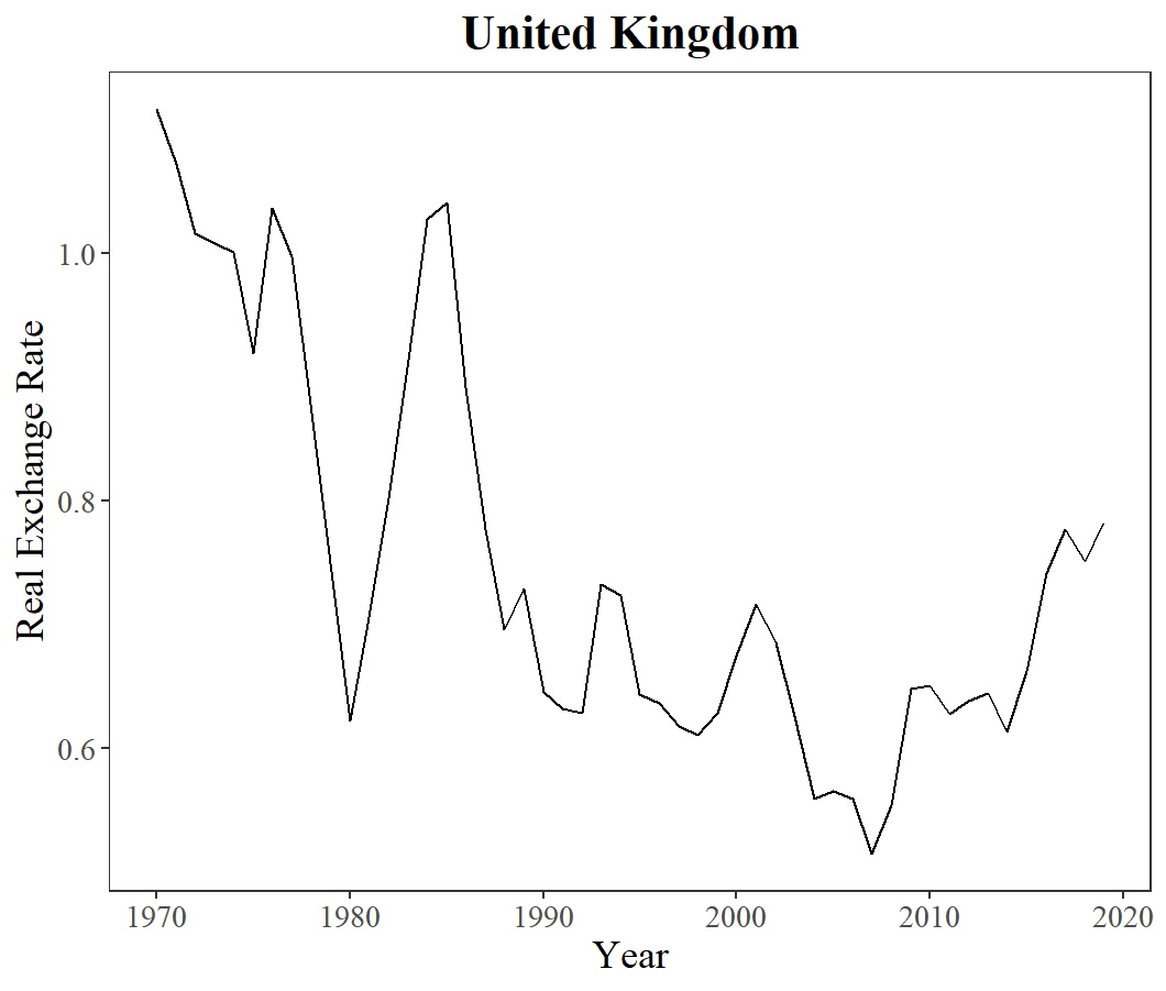
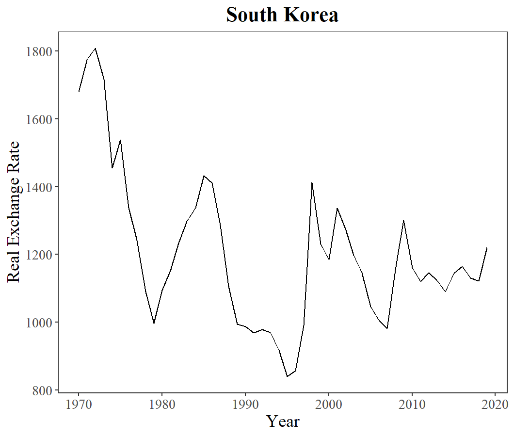
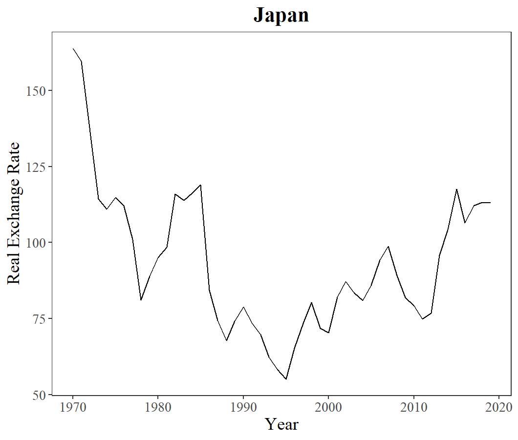
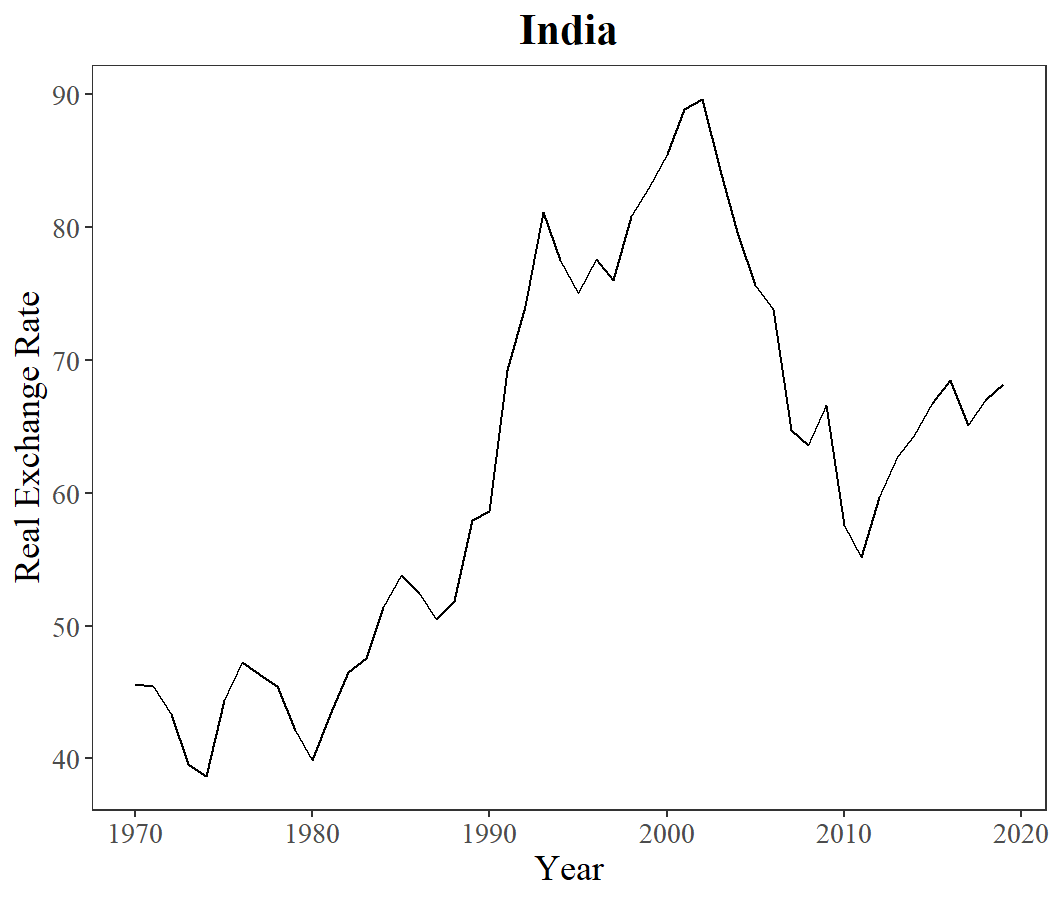
4.1. Absolute purchasing power parity

Absolute Purchasing Powe Parity states that  $$ {RXR}_{i,t}=1$$ , which can be interpreted as the strong version of PPP. The veracity of the equation in  $$ r$$  the real world needs to be investigated. After including real-life error terms of  $$ {RXR}_{i,t}$$ , the equation to be examined is given by:

$$ E{(RXR}_{i,t})=1$$(3)

Where  $$ E{(RXR}_{i,t})$$  is the expected value of a country’s Real Exchange Rate over a certain time period.

The beginning step is generating line charts of the  $$ {RXR}_{i,t}$$  of six selected countries for  $$ t\mathrm{ }ϵ\mathrm{ }\left[\mathrm{1970,2019}\right]$$ , which are America, the United Kingdom, China, Japan, South Korea, India (see Figure 3). As for the horizontal line at  $$ {RXR}_{USA,t}=1$$  for America, it verifies the authenticity of our calculated $$ \mathrm{ }\mathrm{ }{RXR}_{i,t}$$  value, since the Real Exchange Rate for the USD against USD is theoretically one. However, the other charts provide evidence against Absolute PPP. The scales of the vertical axis differ considerably among countries. In addition, based on the mean RXR calculated for the six countries (see Table 4), countries like South Korea, Japan, and India have a mean RXR value significantly larger than 1, while countries like China have a single-digit mean RXR value, and the United Kingdom has a mean RXR value smaller than 1. Following that, a one-sample-t-test to test with hypothesis  $$ H_0:{\mathrm{ }\mu }_i=1\mathrm{ },\mathrm{ }{H}_{\alpha }:{\mathrm{ }\mu }_i\ne 1$$  and a 95% confidence interval (see Table 4) are constructed to test whether the mean RXR value for each country is 1. Among the five countries except America, 1 is contained in none of the 95% confidence intervals, and the p-value is less than any of the common significance levels. As a result, the null hypothesis is rejected and the conclusion is that Absolute PPP does not hold for most countries.

4.2. Relative purchasing power parity

4.2.1. Formula transformation

Relative PPP implies that the purchasing power of a certain currency is constant over a specific time interval. So instead of  $$ {RXR}_{i,t}=1$$ , it is assumed that  $$ {RXR}_{i,t}=k$$ , where k is a constant over a certain time interval, which means the Real Exchange Rate of a country over a specific time interval would fluctuate around a certain value instead of 1.

$$ {RXR}_{i,t}=\mathrm{ }\frac{{XR}_{i,t}\times {PGDP}_{USA,t}}{{PGDP}_{i,t}}=k$$(4)

Taking the natural of each side yields:

$$ \ln \left({XR}_{i,t}\right)+\ln \left({PGDP}_{USA,t}\right)-\ln \left({PGDP}_{i,t}\right)=\ln \left(k\right)$$(5)

$$ \ln \left({XR}_{i,t-1}\right)+\ln \left({PGDP}_{USA,t-1}\right)-\ln \left({PGDP}_{i,t-1}\right)=\ln \left(k\right)$$(6)

Subtract (6) from (5):

$$ \ln \left(\frac{{XR}_{i,t}}{{XR}_{i,t-1}}\right)+\ln \left(\frac{{PGDP}_{USA,t}}{{PGDP}_{USA,t-1}}\right)-\ln \left(\frac{{PGDP}_{i,t}}{{PGDP}_{i,t-1}}\right)=0$$(7)

Given that  $$ \frac{{XR}_{i,t}}{{XR}_{i,t-1}}-1,\frac{{PGDP}_{USA,t}}{{PGDP}_{USA,t-1}}-1$$ ,  $$ \frac{{PGDP}_{i,t}}{{PGDP}_{i,t-1}}-1$$  are only a little bit larger or smaller than 1, the equation can be rewritten as:

$$ {CXR}_{i,t}$$$$ +{Inf}_{USA,t}$$$$ -{Inf}_{i,t}=0$$(8)

Combining the inflation terms,  $$ {Infdif}_{i,t\mathrm{ }}$$ is annotated as the difference of inflation rate ( $$ {Infdif}_{i,t\mathrm{ }}={Inf}_{i,t}-{Inf}_{USA,t}$$ ):

$$ {CXR}_{i,t}={infdif}_{i,t}$$(9)

As shown by the mathematical transformation, Relative PPP implies that there is a direct proportion relationship between the change of exchange rate and the inflation differential for a country at a specific time. Broadly speaking, if the inflation rate of country i goes up more than  $$ \alpha \mathrm{\%}$$  than the USA’s, its exchange rate against the USD should also rise by $$ \mathrm{ }\alpha \mathrm{\%}$$ . This relationship intuitively reflects the constant purchasing power of a type of currency.

4.2.2. Methodology

As stated by the theoretical equation  $$ {CXR}_{i,t}={infdif}_{i,t}$$ , the error term is included and then a linear regression model is built:

$$ {CXR}_{i,t}={{\beta }_0+{\beta }_{1}Infdif}_{i,t}+{\epsilon }_{i,t}$$(10)

The theoretical value of  $$ {\beta }_0$$  and  $$ {\beta }_1\mathrm{ }$$ are both 1. Here one assumption is that there’s no heterogeneity across countries and over time, which implies that  $$ {\beta }_0$$  is the same for each country and each time point. Incidentally, further analysis is conducted afterwards on this assumption. Another assumption is that Cov( $$ {infdif}_{i,t},{\epsilon }_{i,t}$$ )=0, which leaves the estimates unbiased . For the estimation, OLS (Ordinary Least Squares) regression is chosen to estimate the value of  $$ \widehat{{\beta }_0}$$ ,  $$ \widehat{{\beta }_1}.$$  The principle of OLS regression method is to minimize  $$ \sum {\widehat{{\epsilon }_{i,t}}}^2$$ . And OLS estimators are unbiased when there’s no omitted variable bias and fixed effect. Based on our current assumptions, the OLS estimators are unbiased.

4.2.3. 1-year-period pooled OLS regression

The value of  $$ {CXR}_{i,t}$$ , $$ {Infdif}_{i,t}$$  is calculated on the basis of four different time frames: 1-year-period, 5-year- period, 10-year-period, 50-year-period. When constructing a 1-year-period pooled OLS regression, the estimates appear to be abnormal (see Table 5) compared with other time frames. The intercept is small while the slope is very big, and both of them are statistically significant, which is possibly not reliable. Checking the scatterplot (Figure 5), it can be identified that there are several high-leverage point and outliers. These points have high influence on the overall fitted regression line, and they are neither that informative because one economy would not be operating normally at this level. Another reasonable explanation is that they are just simply tying errors. As a result, a quantile-based trimming method is applied to delete some points, given that the quantile value is resistant to outliers.

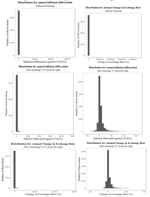
As reported by the histogram of the CXR and Infdif in our 1-year-period dataset (Figure 4), the distributions of both variables show strong skewness to the right, with very few observations deviating a lot from the majority, which is possibly generated by the financial crisis, hyperinflation, or regional conflict. At the same time, a few high-influential points are significantly smaller than the majority. This makes sense since considerable deflation or a decrease in exchange rate has occurred rarely in history. Since the high-influential points are not distributed evenly on both sides, the method chosen is to cut a certain percentage of the observations from the positive end of the number line. Comparing the distributions of CXR and Indfif before trimming and after cutting 0.1% and 1%, the 1% trimming works better for both CXR and Infdif, given that the two distributions of 1% trimming are approximately normal, with slight skewness to the right. Moreover, this skewness can be informative in our future analysis, as it shows what the relationship of CXR and Infdif would be like if there exists high inflation or significant change in the exchange rate, which are not too extreme.

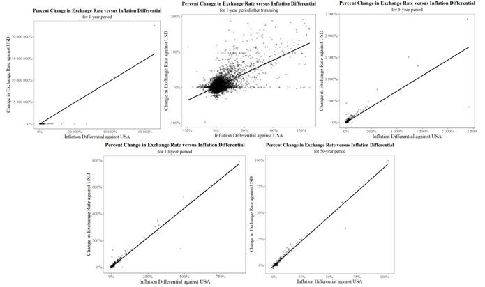
The final method employed is to delete the points with the largest 1% value of CXR or Infdif. In total, 112 observations are deleted from our original dataset for 1-year regression. Since the initial one-year-period dataset is large, containing 9150 observations in total and 183 countries, on average, 0.61 observations are removed from each country, which means there is little information loss. Then, using the trimmed dataset, we run another regression; the 1-year trimmed regression scatterplot in Figure 5 shows a reasonable scale, and the resulting estimates in Table 5 shrink considerably compared with the first one. The estimates are reliable based on the corresponding pattern displayed in the scatterplot.

4.2.4. Pooled OLS regression of other time frames

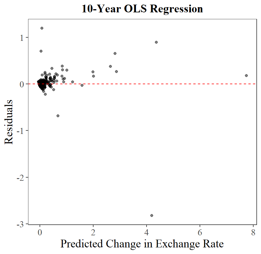
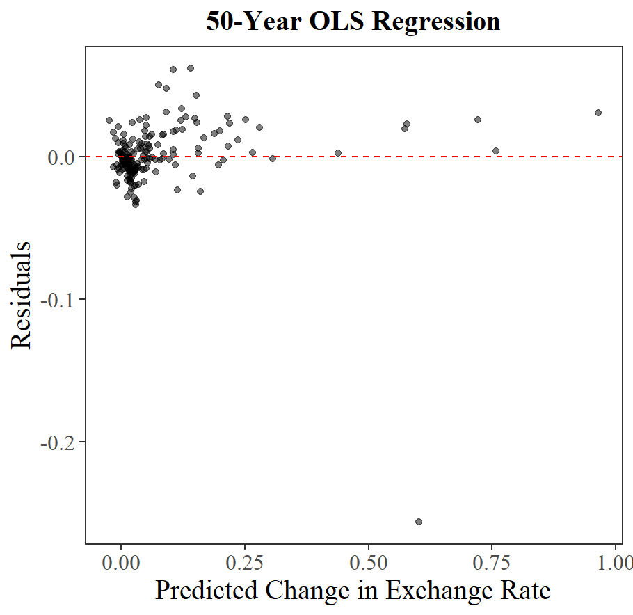
The estimations and scatterplots of running pooled OLS regression based on 5/10/50-year period time frames are obtained and presented (see Table 5 and Figure 5). As indicated in the scatterplot, there are no extremely high influential points like the initial 1-year-period pooled regression model, so there’s no need to perform the trimming method. Otherwise, the risk of losing useful information and degrees of freedom would arise. Additionally, Residue Plots based on the regression model except the initial 1-year pooled one are generated, as shown in Figure 6.

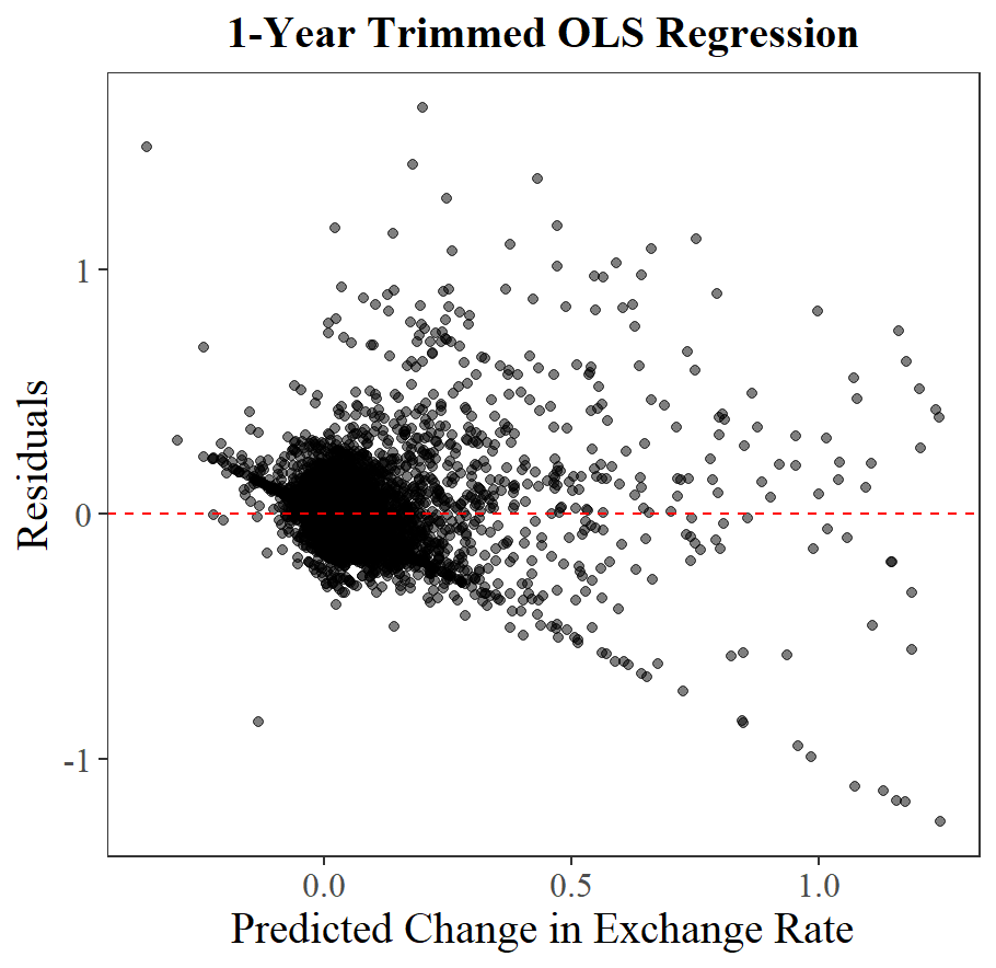
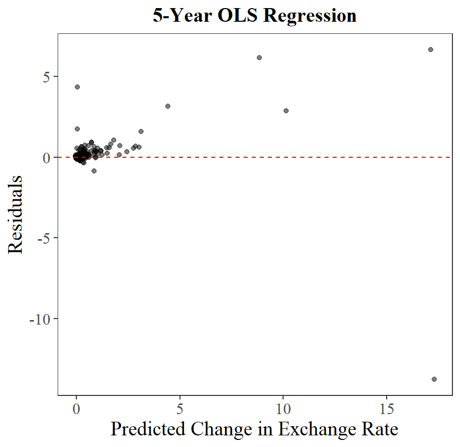
Excluding the initial 1-year erroneous regression, the estimated  $$ \widehat{{\beta }_0}$$ ,  $$ \widehat{{\beta }_1}$$  and Adj- $$ R^2$$  are compared among the other 4 regressions. One finding is that as the time interval becomes larger, the $$ \widehat{{\mathrm{ }\mathrm{ }\beta }_0}$$ ,  $$ \widehat{{\beta }_1}$$  gradually converge to their theoretical value:  $$ \widehat{{\mathrm{ }\beta }_0}$$  shrinks from 0.9533 to -0.0003, approaching its theoretical value 0, and  $$ \widehat{{\beta }_1}$$  grows from 0.7520 to 0.9344, approaching 1. Moreover, the significance level of the intercept  $$ \widehat{{\mathrm{ }\beta }_0}$$  decreases from highly significance to insignificance, thus null hypothesis  $$ {\mathrm{ }\beta }_0$$ =0 cannot be rejected over 50-year period. Besides, the Adj- $$ R^2$$  values simultaneously improves as the time interval grows larger. This outcome shows that the relationship between CXR and Infdif is becoming stronger and clearer as the time interval expands. Although given the significance of the intercept and slope, a relationship do exist in short time intervals like one year. Relative PPP does not hold true for one-year period since the relationship is too weak (Adj- $$ R^2<0.5$$ ), which is due to short-run fluctuations and reacting time required for the dynamics between exchange rate and inflation rate. As a result, it is concluded that Relative PPP can not hold true over one year. But 5 years or more allows Relative PPP to hold true, and 50-year period can enable it to hold accurately.

In accordance to the residue plots (Figure 6), there are no obvious trends on those residue points. This confirms that there is no autocorrelation of nonlinearity problems.

4.2.5. Grouped OLS regression based on openness

Recall that when using pooled OLS regression method, one of the assumptions is that there’s no heterogeneity among countries. Now this assumption is re-examined, by categorizing the 183 countries into different groups based on certain traits. And then different time-frame regression is constructed upon each group. The question is that whether there is significant difference between the two groups’ estimates within one data frame, which may indicate our initial regression model’s first assumption is violated and can be improved by running this grouping OLS regression. Countries excluding the OPEC members are assigned into Open_Group and Other_Group based on their openness to trade. The Open_group is considered to be relatively open-trading economy, and Other_group contains the rest.

The steps of grouping countries are:

1). Exclude the OPEC country from the overall dataset of each time frame.

2). Select the Open_Group countries based on the criteria:

$$ \stackrel{-}{\frac{{Q\_X}_{i,t}+{Q\_M}_{i,t}}{{Q\_GDP}_{i,t}}}$$$$ >0.5\mathrm{ }\mathrm{ }\mathrm{ }\mathrm{ }\mathrm{ }\mathrm{ }\mathrm{ }\&\mathrm{ }\mathrm{ }\mathrm{ }\mathrm{ }\mathrm{ }\mathrm{ }\mathrm{ }\stackrel{-}{\mathrm{ }\frac{{Q\_X}_{i,t}}{{Q\_M}_{i,t}}}$$$$ ϵ\left(\mathrm{0.6,1.65}\right)$$(11)

The outcomes of regression based on different time frames are presented on Table 6:

Based on our regression outcomes, the Adj- $$ R^2$$  values are similar between the two groups within each time frame. Meanwhile, the estimated coefficients are similarly close to 0 and 1. As a result, the conclusion drawn is that there is no heterogeneity between countries of different levels of openness within each time frame. In addition, since 13 OPEC countries are excluded from our dataset, and most of these countries have many extreme Infdif and CXR values due to their dependence on oil. Consequently, when constructing the 1-year OLS regression, the estimates are not as anomalous as before.

4.2.6. Grouped OLS on PPP theory based on exchange rate policies

Besides grouping based on openness to trade, the aim of this section is to find out the effect of exchange rate policies on the validity of PPP Theory. In the set of data, some countries, such as Aruba, have a fixed exchange rate with the US through the 50 years analysed, while 90 countries had a floating exchange rate throughout. In addition, some countries, such as South Korea during the Asian financial crisis 1997, changed from a fixed to a floating exchange rate system, and other countries, such as the Bahamas in 1993, changed from a floating to a fixed exchange rate policy to ensure economic stability. Figure 7 is a graph of all countries distributed by the percentage of years with zero annual exchange rate change from 1970 to 2019, or the percentage of years with fixed exchange rate with the US. We, therefore, divide the data into two groups, one of countries and years with fixed exchange rates, and the other with floating exchange rates. Data from countries such as South Korea and the Bahamas will be split into two different groups based on the year.

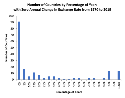
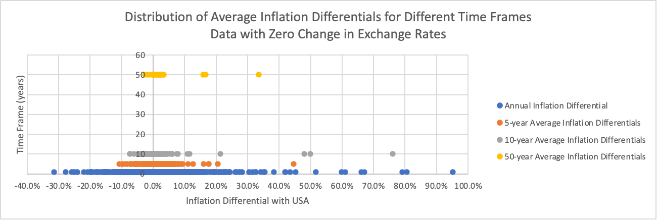
Figure 8 illustrates average inflation differentials against the US from countries with a fixed exchange rate against the US. The figure compares the distribution of annual, 5-year, 10-year, and 50-year average inflation differential. Countries with fixed exchange rates against the US in shorter annual periods tend to have higher fluctuations in inflation differentials against the US. In contrast, as the period increases, the average fluctuation tends to decrease, with the 50-year-average inflation differentials being 2.74% average and the standard deviation being 6.32%. This indicates that for countries with fixed exchange rates against the US, the PPP theory tends to hold over more extended periods. The result is also proof towards the Unholy Trinity of Exchange Rates [11], stating that countries cannot simultaneously have a fixed exchange rate, free capital movement, and sovereign monetary policy. Over more extended periods, the converging average inflation differentials demonstrate that countries with fixed exchange rates against the US tend to lose monetary independence, validating the theory.

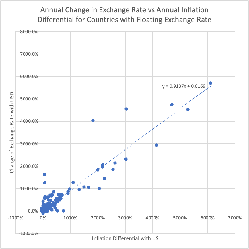
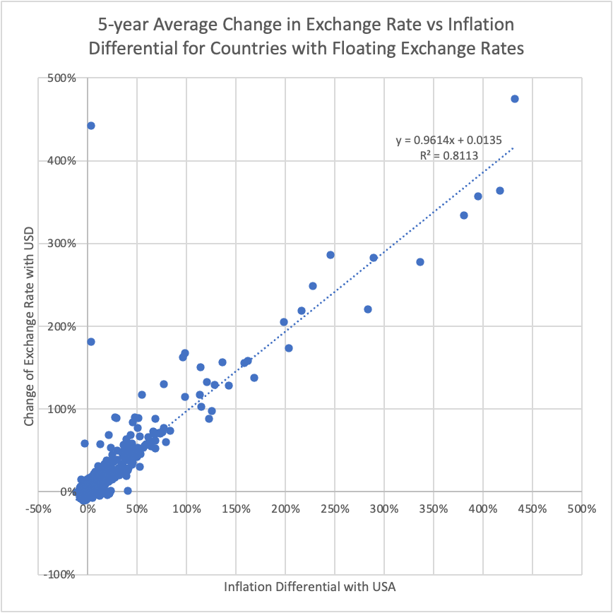
For the group of countries with floating exchange rates, Figure 9 shows that the PPP theory tends to hold in shorter time periods compared to the group with fixed exchange rates. Annual and five-year-average graphs of inflation differential against exchange rate have relatively high R-squared values (0.8113) and a slope close to 1 (0.9614 and 0.9137).

5. Economic growth model

Relative PPP indicates that government intervention can manipulate a country’s currency's real exchange rate over the short run. Further exploration is needed to determine whether a relationship exists between economic growth and real exchange rates. The measurement of economic growth is the GDP growth rate. Since the Absolute PPP does not hold, the Real Exchange Rate of different countries fluctuates around different levels. Hence, two distinct techniques are employed to normalize the level of RER in different countries. The main methodology is constructing a model to predict economic growth and incorporating the transformed RXR term to identify its effect.

5.1. Grouped economic growth model based on OECD membership

5.1.1. Model construction

To explain the result more accurate, it is initially decided to separate the dataset into two groups: OECD countries and non-OECD countries, where OECD members are mainly countries that have developed, mature and appropriate economic system. The original model chosen for both groups is:

$$ Growt{h}_{i,t}={\beta }_0+{\beta }_{1}RGDPC{H}_{i,t-1}+{\beta }_{3}UDERVA{L}_{i,t}+f_i+f_t+{\epsilon }_{i,t}$$(12)

Where  $$ f_i,f_t$$  are added using fixed effects estimation, to make up for the heterogeneity across individuals and time. To clarify about the regressors, one regressor  $$ RGDPC{H}_{i,t-1}$$  is calculated by:

$$ RGDPC{H}_{i,t}=$$ ( $$ \frac{Q-GDP\_(i,t)}{Populatio{n}_{i,t}}$$(13)

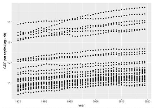
Here RGDPCH in the previous year is used, the purpose of which is to solve the problem of trend within the RGDPCH data (see Figure 10). Using RGDPCH of prior year, the influence of present condition on the future growth can also be detected.

Another regressor  $$ UDERVA{L}_{i,t}$$  is an indicator for Real Exchange Rate. Specifically, to account for the fact that non-tradable goods are cheaper in poorer countries (Balassa–Samuelson effect [12,13]), a regression using fixed effects estimation relating  $$ lnRX{R}_{i,t}$$  and  $$ RGDPC{H}_{i,t}$$  are first constructed to compensate for the difference in Real Exchange Rate caused by different development levels.

$$ lnRX{R}_{i,t}={\alpha }_0+{\beta }_{1}RGDPC{H}_{i,t}+f_i+{\epsilon }_{i,t}$$(14)

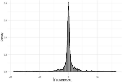
Then the formula of the natural log UNDERVAL is given by:

$$ lnUNDERVA{L}_{i,t}=\mathrm{l}\mathrm{n}\left(RX{R}_{i,t}\right)-\mathrm{l}\mathrm{n}(\widehat{RX{R}_{i,t})}$$(15)

Figure 11 shows the histogram of  $$ UDERVA{L}_{i,t}$$ . From the two distributions, it can be identified that the distribution of natural log of the UNDERVAL is normal. On top of that, two regressors are then selected to add to the original model for more precise information: the investment proportion in the nominal GDP (16) and the openness of a country to trade (17).

$$ {IGDP}_{i,t}=\frac{V-I_{i,t}}{V-{GDP}_{i,t}}\mathrm{ }$$$$ \mathrm{ }$$(16)

$$ {\mathrm{ }Tradeopen}_{i,t}=\frac{V-m_{i,t}+V-x_{i,t}}{V-{GDP}_{i,t}}$$(17)

Eventually, the final model of economic growth for both groups is determined as:

$$ Growt{h}_{i,t}={\alpha }_{i,t}+{\beta }_{1}RGDPC{H}_{i,t-1}+{\beta }_{2}UDERVA{L}_{i,t}+{\beta }_{3}tradeope{n}_{i,t}+{\beta }_{4}IGD{P}_{i,t}+f_i+f_t+{\epsilon }_{i,t}$$(18)

5.1.2. Regression outcomes

First, a fixed effects regression is fitted on the OECD-country group based on the final model. (see Table 7)

According to the result, although all of the coefficients are significant, inspection is still required to determine potential problems. Subsequently, the model is refined using statistical methods to try to reduce the impact of several other issues. To begin with, heteroscedasticity is checked by implementing the Breusch-Pagan test to detect it (see Table 8), setting the significance level  $$ \alpha =0.05$$ . The test yields a  $$ p-value$$  less than 0.05, contradicting the null hypothesis; thus, a heteroscedasticity problem exists.

To solve the problem introduced by heteroscedasticity, the clustered standard error is used. After addressing the heteroscedasticity, the modified coefficient is available (Table 9). It can be observed that the coefficient of lnUNDERVAL becomes insignificant with an increase in standard error.

Next, the fixed effect model focuses on non-OECD countries' economic growth. Generally speaking, the same procedure is replicated to fit our model on Non-OECD countries, which includes (1) determining the normality of lnUNDERVAL’s distribution for Non-OECD countries(see Figure 11), (2) fitting the fixed effect model and managing to address the problem such as heteroscedasticity. Overall, the result shown in Table 10 demonstrates a similar effect of specific economic policies. However, this result is noticeably different from the previous group, mainly because the Non-OECD group does not have heteroscedasticity within the model, given that the p-value is obviously above 0.05 (see Table 11).

Comparing the two groups’ regression outcomes after BP-test correction, the insignificance of lnUNDERVAL shows that undervaluation does not play a noticeable role in the contribution of economic growth in this model. However, other regressors are informative in the model building. Negative RGDPCH shows that the richer a country is, the more challenging it is to keep a high growth rate, and this effect is more significant in OECD countries. A higher trade open coefficient in OECD countries implies that international institutions like the OECD and WTO can help countries grow. In both groups, investment is the highest, which means that investment is essential for growth.

5.2. Pooled economic growth model

The first model is recognized as having limitations. There are multiple regressors, and some of them can be correlated. For example, lnUNDERVAL and tradeopen may increase the standard error of lnUNDERVAL’s coefficients. Except for IGDP, other estimations are similar between OECD and Non-OECD groups. To concentrate more on the effectiveness of the exchange rate and reduce the effect of potential multicollinearity, we removed the investment and trade as a measurement of the economy. Combining the two groups to run a pooled regression on all countries will simplify the model. Furthermore, the previous model is constructed using an untrimmed one-year data frame, which takes the risk of being influenced by high-leverage points and short-run instability. Since in a 5-year period, Relative PPP holds moderately, and instability can be alleviated, as indicated in the PPP investigation part. 5-year is chosen in this model to be a more proper time frame.

5.2.1. Feature engineering

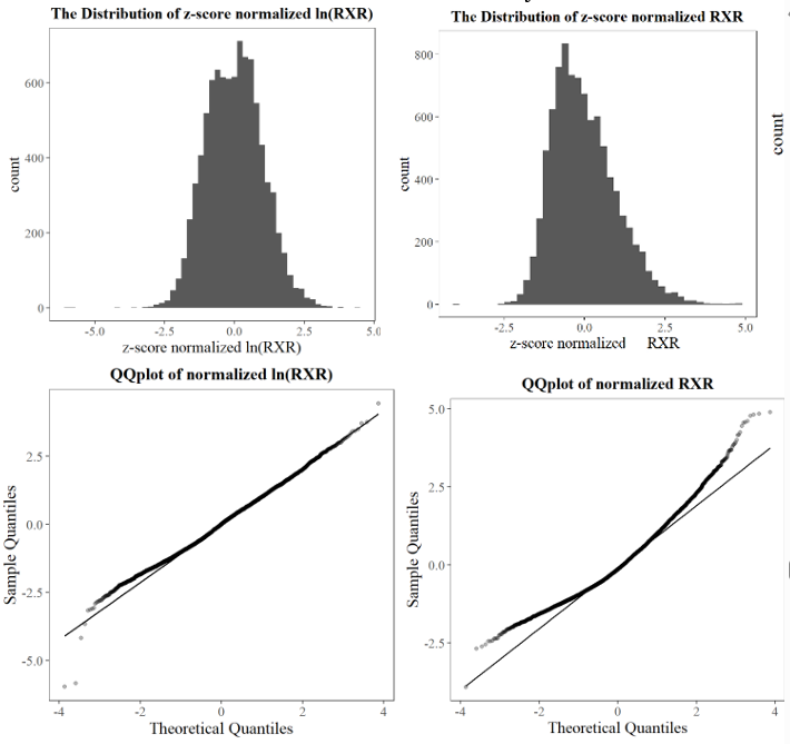
Firstly, a variable that represents the appraisal of the exchange rate is modified. Z-score normalized real exchange rate (Referred to as Norm-RXR later) is introduced to standardize the RXR. This method uses the mean Real Exchange Rate as a marker for the country’s intrinsic Real Exchange Level (caused by its productivity of tradable gooda) regardless of government intervention. Comparing the histograms and QQ-plots of Norm-lnRXR and Norm-RXR (Figure 12), the distribution of Norm-lnRXR is closer to normal distribution, so we use Norm-lnRXR as a regressor.

$$ Norm{\ln \left(RXR\right)}_{i,t}=\frac{{\ln \left(RXR\right)}_{i,t}-\stackrel{-}{l{n\left(RXR\right)}_i}}{{\sigma }_{{\ln \left(RXR\right)}_i}}$$(19)

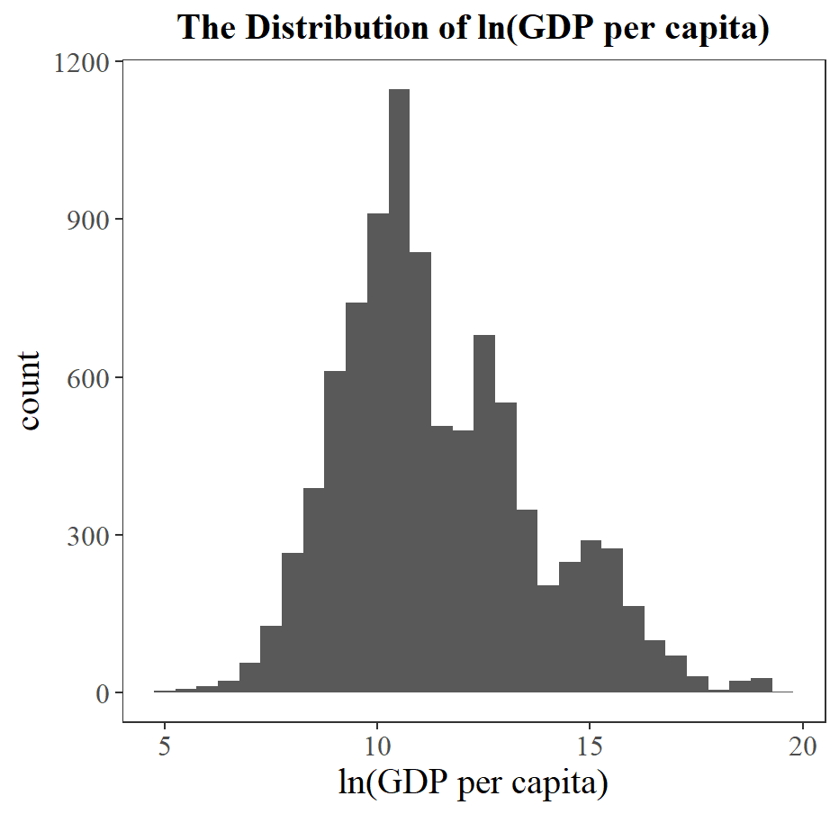
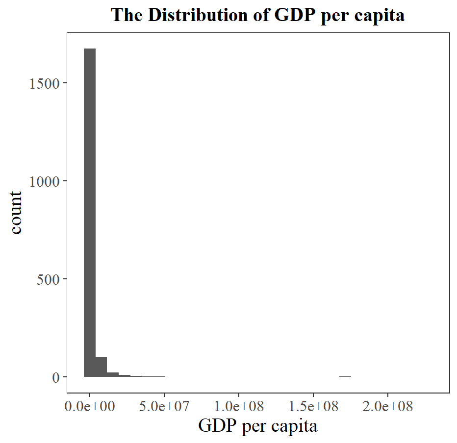
Transformation is also performed to map RGDPCH into lnRGDPCH, since the distribution for lnRGDPCH is closer to normal distribution (see Figure 13).

Plus, a new variable  $$ gov\mathrm{ }in{v}_{i,t\mathrm{ }}$$ is added in order to measure the government involvement level in the economy:

$$ gov\mathrm{ }in{v}_{i,t}=\frac{V-G_{i,t}}{V-GD{P}_{i,t}}$$(20)

5.2.2. Model revision

According to the selected variables and time frame, the work here employs fixed/random effects to estimate the coefficients of the following three models, progressing from the simple to complex:

$$ {Growth}_{i,t}=f_i+f_t+{\alpha }_{i,t}+{{\beta }_{1}Norm\mathrm{ }lnRXR}_{i,t}+{\epsilon }_{i,t}$$(21)

$$ Growt{h}_{i,t}=f_i+f_t+{\alpha }_{i,t}+{\beta }_{1}Norm\mathrm{ }lnRX{R}_{i,t}+{\beta }_{2}lnRGDPC{H}_{i,t-1}+{\beta }_3\left(Norm\mathrm{ }lnRX{R}_{i,t}\times lnRGDPC{H}_{i,t-1}\right)+{\epsilon }_{i,t}$$(22)

$$ Growt{h}_{i,t}=f_i+f_t+{\alpha }_{i,t}+{\beta }_{1}Norm\mathrm{ }lnRX{R}_{i,t}+{\beta }_{2}lnRGDPC{H}_{i,t-1}+{\beta }_3\left(Norm\mathrm{ }lnRX{R}_{i,t}\times lnRGDPC{H}_{i,t-1}\right)+{\beta }_{4}gov\mathrm{ }involv{e}_{i,t}+{\epsilon }_{i,t}$$(23)

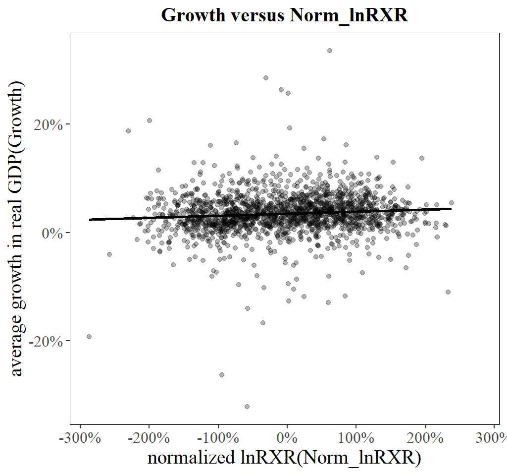
we first fit the Model (21) alone with the Norm-lnRER and GDP growth, and random effects estimation is used, according to the output of Hausman test (Table 16) that the null hypothesis is not rejected. The result is given by Table 12 and we also generate a scatterplot relating Growth and Norm-lnRXR (see Figure 14).

Furthermore, the observations are split into two groups based on the time (before or after 2000), and random effects regressions are carried out based on Model (21) for both groups. While the coefficient of Norm-lnRXR remains highly significant (***) in the after-2000 groups, the significance level of that in the before-2000 groups drops to two stars. Given the unstable international relations like the Cold War and economic crises such as the oil crises, this outcome potentially stems from a turbulent global economic situation that interferes with with trading.

Secondly, in Model (22) the feature RGDPCH is added, for the purpose to measure the influence previous state of countries’ economy on the future stages. This work also incorporates an interaction term on RGDPCH and Norm-RER, so the effect when both variables interact with each other can be examined.

The result of random effects model is presented on Table 14.

From the comparison of two models, it can be observed that R-squared has been improved as well as the adjusted R-squared, which indicates the progress in the model. However, the significance level of Norm-lnRXR falls, caused by the complexity of the model. To further fit this model, one more feature  $$ gov\mathrm{ }in{v}_{i,t}$$  is included to construct Model (23). Utilizing the  $$ gov\mathrm{ }in{v}_{i,t}$$  contributes to the examination about what effect the policies and actions directed by governments have. The proportion of government expenditure in turns can reflect the participation and energy of private sector and further reveal the economic trends. From the result of fixed effect estimation of Model (23) presented on Table 15, it’s relatively clear that gov-involve and RGDPCH are very significant in the model. And the sign of Norm-lnRXR’s coefficient is positive, but it’s insignificant. Through this type of feature engineering the model’s quality has been improved given the rising  $$ R^2\mathrm{ }$$ as well as Adj- $$ R^2$$. Yet, a conclusion can not be drawn until we compare each other’s AIC.

5.2.3. Model improvement

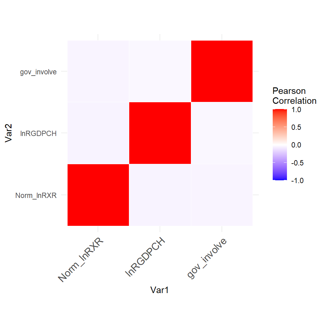
After constructing the revised three models, it is considered that the significance level of Norm-lnRXR depends on the complexity of the model, which may possibly result from multicollinearity. In order to determine the final variables for our regression model, several statistical methods are employed, for the purpose of detecting several problems such as heteroscedasticity, endogeneity and multicollinearity, which are covered in this subsection. To start with, multicollinearity is checked using the correlation heat-map (Figure 15). From the correlation heat-map, it can be learned that the correlation between each pair of variables is slight and unimportant, so the concern can be withdrawn.

BP test is then used to check the existence of heteroscedasticity. Given the p-value that is beyond 0.05, it can be concluded that there is no heteroscedasticity (see Table 17).

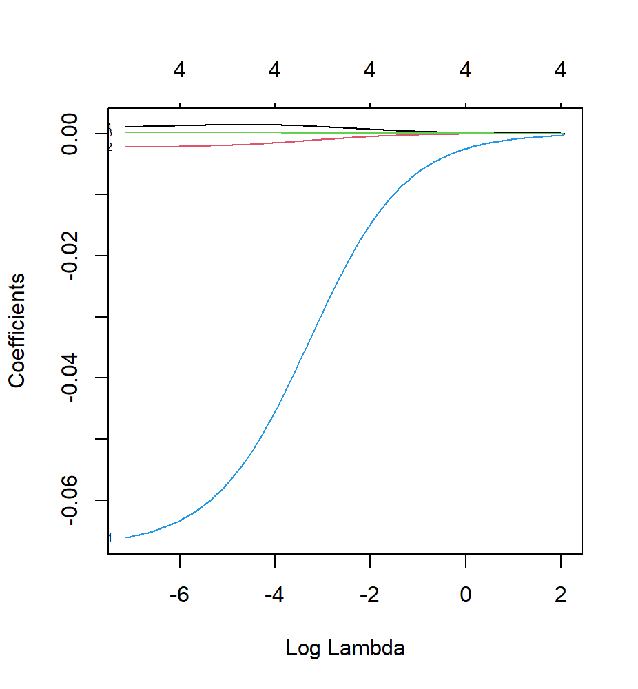
The endogeneity part included in the process of selecting fixed or random effect model, so no more specific test is conducted here. Finally, the procedure of regularization is executed applying Ridge regression in order to further refine Model (23). Choosing the best λ value 0.002 (Figure 16), the regression result suggests that all four variables should be considered, and the coefficient of Norm-lnRXR is positive (see Table 18), meaning that increasing the real exchange rate can make a contribution to the economic growth.

6. Conclusion

The paper carefully and subtly analyzes the interesting negative link between RER undervaluation and economic growth, empirically grounded within the theoretical setting of PPP. This paper tests the validity of absolute and relative PPP very rigorously across different sets of economies and time frames, providing important insights that add meaningfully to the debate in international macroeconomics. First, it confirms that absolute PPP does not hold across the selected countries by showing significant deviations in the real exchange rate from unity. The statistical rejection of the absolute PPP stresses the inadequate assumption of a common price level across economies, thus challenging the traditional view that exchange rates purely reflect relative price differentials. These deviations are not simple statistical aberrations but are reflective of more fundamental differences in the structure of these economies, such as differing degrees of market integration, divergent inflationary environments, and distinct macroeconomic policies—factored in. This finding makes very clear how important it will be to include country-specific factors when seeking an understanding of exchange rates, tending to emphasize that Absolute PPP is theoretically most appealing but is incapable in practice of taking into account the myriad of factors that actually influence exchange rate behavior.

In an empirical perspective, alternatively, it confirms the hypothesis of the Relative PPP for long time periods; that is, changes in exchange rates are proportional to inflation differentials between countries examined, which can be found really close when analysis is done over five years or more. According to the pooled OLS regressions conducted, it is clear that the econometric analysis not only suggests but also shows clearly that even if there is some noise caused by short-term fluctuations, exchange rates really do adjust according to the trend of inflation over a long period of time. The fact that the estimated coefficients of the regression all turn out to be significant, with high adjusted R-squared values, confirms that Relative PPP holds very robustly in the long run; it is capable of providing a useful general framework for understanding the dynamics of exchange rates over an extended period, especially within the setting of international macroeconomic analysis.

The research into RER undervaluation and its effect on economic growth paints a more nuanced picture. Such econometric models, with state-of-the-art feature engineering that includes normalized RER and interaction terms with GDP per capita growth, permit granular and precise estimation of these effects. It is possible to deduce that the undervaluation of the RER actually does spur economic growth through the boost in export competitiveness. This effect is very strong in non-OECD countries where undervaluation played a compensating role for structural weaknesses and shallower industrial diversification. The findings suggest that a deliberately undervalued currency would be one stimulus underpinning growth in such economies since it moots competitive exports and higher GDP growth rates.

However, the sustainability of such a policy is l growthooked at with a critical view. According to the study, the benefits of RER undervaluation depend on a fine trade-off between short-term gains and long-term economic stability. While in OECD countries, where economic structures are more mature and the financial system more robust, RER undervaluation has a minor contribution to growth with greater risks for inflation, accumulation of external debt, and financial instability. These findings suggest that exchange rate policy has to be ordered in broader economic and institutional contexts. The rigor in methodology and the contribution that the workings bring to the study are apparent, as reflected in these state-of-the-art econometric techniques: the application of fixed and random effects models and interaction terms picking up nuanced effects of RER undervaluation across a variety of economic contexts. Such methodological contributions not only naturally enhance the accuracy of the findings for this current study but also provide a template for future research in his area. The results affirm that while RER undervaluation can be strategically used to spur economic growth, especially in developing economies, its effectiveness is moderated by the level of economic development and the prevailing economic conditions.

The overall contribution of this research toward a better understanding of exchange rate policy is such, as it will go on to provide a theoretically detailed and empirically grounded analysis of the role RER undervaluation can play in economic growth. While Relative PPP provided a remarkably solid framework for the long-term characterization of exchange rate dynamics, undervaluation as an overarching strategy for promoting economic growth is the most cautious of all policies. Policies need to be tailored according to the specific country's economic and institutional context, considering trade-offs that may occur between short-term competitiveness and long-term economic stability. Such models should be further refined in future studies through the inclusion of more disaggregated data and an investigation of how the exchange rate policy tools interact with other macroeconomic variables.

Acknowledgment

Naoki Nanasha, Jiaming Zhang, Yijun Zou, and Sankuai, Gao, contributed equally to this work and should be considered co-first authors.

References

[1]. Kausar, R. and Zulfiqar, K. (2017) 'Exchange Rate Volatility and Productivity Growth Nexus in Selected Asian Countries', Pakistan Economic and Social Review, 55(2), pp. 595-612. [Available at: https: //www.jstor.org/stable/10.2307/26616727 (Accessed: 17 August 2024)].
[2]. Minford, P. (1981) 'The Economic Consequences of Exchange Rate Regimes', Economic Journal, 91(361), pp. 138-152.
[3]. Mark, N.C. (1995) 'Exchange Rates and Fundamentals: Evidence on Long-Horizon Predictability', American Economic Review, 85(1), pp. 201-218.
[4]. Cassel, G. (1918) 'The Present Situation of the Foreign Exchanges', The Economic Journal, 28(112), pp. 413-428.
[5]. Corbae, D. and Ouliaris, S. (1988) 'Cointegration and Tests of Purchasing Power Parity', The Review of Economics and Statistics, 70(3), pp. 508-511.
[6]. Rogoff, K. (1996) 'The Purchasing Power Parity Puzzle', Journal of Economic Literature, 34(2), pp. 647-668.
[7]. Sarno, L. and Taylor, M.P. (2002) 'Purchasing Power Parity and the Real Exchange Rate', IMF Staff Papers, 49(1), pp. 65-105.
[8]. Jahan-Parvar, M.R. and Mohammadi, H. (2011) 'Oil Prices and Real Exchange Rates in Oil-Exporting Countries: A Bounds Testing Approach', The Journal of Developing Areas, 45(1), pp. 313-322.
[9]. Dupuis, D.J. and Victoria-Feser, M.-P. (2013) 'Robust VIF Regression with Application to Variable Selection in Large Data Sets', The Annals of Applied Statistics, 7(1), pp. 319-341.
[10]. Fernholz, R., Fernandez, R., and Kletzer, K. (2015) 'Exchange Rate Manipulation and Currency Wars', Journal of Economic Dynamics and Control, 52, pp. 95-117.
[11]. Mundell, R.A., 1963. Capital mobility and stabilization policy under fixed and flexible exchange rates. Canadian Journal of Economics and Political Science, 29(4), pp.475-485.
[12]. Balassa, S., 1964. The purchasing power parity doctrine: A reappraisal. Journal of Political Economy, 72(6), pp.584-596.
[13]. Samuelson, P.A., 1964. Theoretical notes on trade problems. Review of Economics and Statistics, 46(2), pp.145-154.
Cite this article
Nanasha,N.;Zhang,J.;Zou,Y.;Gao,S. (2025). Real Exchange Rate in the Measurement of Purchasing Power Parity and Its Long-term Impact on Economic Growth. Advances in Economics, Management and Political Sciences,198,71-96.
Data availability
The datasets used and/or analyzed during the current study will be available from the authors upon reasonable request.
Disclaimer/Publisher's Note
The statements, opinions and data contained in all publications are solely those of the individual author(s) and contributor(s) and not of EWA Publishing and/or the editor(s). EWA Publishing and/or the editor(s) disclaim responsibility for any injury to people or property resulting from any ideas, methods, instructions or products referred to in the content.
About volume
Volume title: Proceedings of the 3rd International Conference on Financial Technology and Business Analysis
© 2024 by the author(s). Licensee EWA Publishing, Oxford, UK. This article is an open access article distributed under the terms and
conditions of the Creative Commons Attribution (CC BY) license. Authors who
publish this series agree to the following terms:
1. Authors retain copyright and grant the series right of first publication with the work simultaneously licensed under a Creative Commons
Attribution License that allows others to share the work with an acknowledgment of the work's authorship and initial publication in this
series.
2. Authors are able to enter into separate, additional contractual arrangements for the non-exclusive distribution of the series's published
version of the work (e.g., post it to an institutional repository or publish it in a book), with an acknowledgment of its initial
publication in this series.
3. Authors are permitted and encouraged to post their work online (e.g., in institutional repositories or on their website) prior to and
during the submission process, as it can lead to productive exchanges, as well as earlier and greater citation of published work (See
Open access policy for details).