1.  Introduction

Climate change is, most evidently, a global challenge with deep implications and consequences, cutting across. The large magnitude of the problem can be seen in the 2022 Intergovernmental Panel on Climate Change report, which has laid down that even under full implementation, under current carbon reduction policies, global temperatures are likely to rise by 3.2°C before 22^nd century—an upsurge that poses severe natural, social, and economic risks. According to the World Economic Forum Global Risks Report 2023, climate-related risks have finally turned into critical risks to economic stability. Climate issues are now placed on the list among risks such as natural disasters, extreme weather events, and the breakdown of global agricultural systems. These effects come out in financial markets, especially those of agricultural futures, from where changes in weather patterns can strongly affect the supply chain, market volatility, and investors' sentiments. We want to understand these dynamics, relevant to the assessment of resilience and adaptability in the agricultural futures market in the face of climate uncertainty and potential policy responses to altered environments.

In discussing the role of climate change, agriculture represents one of the most critical sectors of the national economy and has strong links with the most fundamental needs related to, for example, food security, economic resilience and social stability. The impacts of climate change on agricultural markets are broad and complex in nature. Direct outcomes from natural disasters, such as hurricanes and droughts, often lead to price volatility and the disruption of supply chains after adversely affected agricultural production. Agricultural produce, as elementary commodities, depend on climatic conditions for production and are thus sensitive to changes in the environment [1]. Furthermore, agricultural products have strong financial characteristics. Financial derivatives related to it are thus sensitive to changed climate policy and investor sentiment regarding climate risks. Regulatory changes or extreme weather events can quickly change market dynamics, ultimately affecting investor behavior and thus potential returns in agricultural markets.

​ The occurrence of extreme weather events and their impacts has been occurring more frequently under the process of global climate change intensification. This situation has caused great concern about its effects on agricultural markets. Soybeans, among the important sources of proteins and fats, are grown on several continents and are particularly sensitive to climate changes. Extreme weather events, such as hurricanes, droughts, and storms, would greatly change conditions for soybean growth and harvesting, hence affecting yields and making it very hard to predict market outcomes. In most cases, future uncertainties increase the volatility of prices. All these affect not only the stakeholders that are directly involved in the terms of the soybean market but also a more general economy dependent on agricultural exportations.

Though so many studies display the effect of climate change on agricultural production, yet so few concentrate on the financial implications of climate factors for agricultural futures. The current research paper will contribute to fill this gap by studying the impacts of Climate Policy Uncertainty (CPU) and the Climate Physical Index (CPI) on the soybean futures' volatility.

2.  Literature review

Volatility in the prices of agricultural commodities, and more specifically in soybean prices, is highly dependent on climate-related factors. Of the very many models available out there, this study adopts the GARCH-MIDAS model, which combines high-frequency data from financial markets with low-frequency data on climate variables. This literature review focuses on synthesizing work that has been done regarding how Climate Policy Uncertainty (CPU) and Climate Physical Index (CPI) affect the realization volatility of soybean futures prices (RV).

​ Climate policy uncertainty (CPU) was one of the most influential exogenous factors that affected the financial markets in general and the agricultural commodities sector in particular. Guo et al. developed an index for CPU based on emerging text-mining methods and showed that the identified CPU significantly affected agricultural product prices as a key channel—particularly, influencing investor sentiment and market volatility on a short-term basis [2]. Similarly, Baker et al. and Hong et al. imply that increased market volatility stems from economic policy uncertainty regarding climate policy [3-4]. The most recent evidence of such has been demonstrated by Lee et al. and Nordhaus, showing that changes in climate policy change and influence energy and agricultural markets dramatically due to regulatory uncertainty [5-6]. As Jin and Cheong point out, markets are global nowadays, so it is demonstrated how, due to such a factor as CPU, the prices of agricultural commodities have become more volatile in swiftly developing Asian economies [7]. Combined, these studies all point to the need for developing effective risk management strategies, which would underpin the notion of market stability without undermining sustainable economic growth within a complicated policy framework.

As a matter of fact, the CPI summarizes what the climate is doing to the futures markets, counting risks from extreme weather events like droughts, floods, and heatwaves that directly affect agricultural production and prices. Auffhammer and Carleton and Hsiang study have established that such weather events can greatly lead to swings in agricultural commodity prices [1,8]. Auffhammer identified that in periods of severe droughts and prolonged heat waves, crop yields are disrupted, leading to market volatility [8]. Carleton and Hsiang highlighted that floods and hurricanes are also seen to destroy crops and disrupt supply chain infrastructure, something that eventually results in higher price instability. Matiu et al. noted that heat and drought cause a decrease in global soybean production by 12.4%, causing supply shortages and price spikes [9]. Lobell et al. demonstrated that even small rises in temperatures had the potential to cause huge reductions in the yields of key crops globally, such as maize, wheat, and rice [10]. In 2016, Lesk et al. concluded that extreme weather is the most influential of all the factors contributing to market price volatility in agriculture [11]. Schlenker and Roberts showed a very high sensitivity of crops to temperature changes, such that severe heat waves in the United States could lead to drastic declines in crop yields [12]. Together, these studies demonstrate the importance of embedding CPI in economic models to have them more accurate and reliable for predicting agricultural commodity prices, hence in helping develop strategies to mitigate these risks.

​Realized Volatility (RV) tracks the actual pricing movement that takes place over time and is considered an important means of understanding changes in the market. Luo et al. and McAleer and Medeiros highlighted how RV is significant in reflecting market behavior and its usefulness in forecasting models [13-14]. By mixing it with Climate Policy Uncertainty (CPU) and Climate Physical Index (CPI), it enables comparative analysis of both short-term and long-term market effects.

Engle et al. developed the GARCH-MIDAS model, which offers an ideal and robust structure for predicting volatility [15]. In doing this, high-frequency market data is mixed with low-frequency macroeconomic variables, which makes the framework be in a position of allowing mixed-frequency data to ensure the capturing of the effect of slow-changing economic variables on financial markets. Recent studies have shown that this model has been successfully applied to the prediction of market volatility in various financial environments. For instance, by employing a GARCH-MIDAS model to study the dynamic correlation of economic policy uncertainty with financial stress, Raza et al. found their model to provide results full of prospect in handling complex multifrequency datasets [16]. The authors applied the model to forecast stock market volatility, showing effectiveness in combing macroeconomic indicators across different timescales [17]. In another practical validation, Fang et al. reported an application of the model in the prediction of stock market volatility; where the model confirmed to be well suitable for using data of mixed frequencies and improving forecast accuracy [18]. As an example, in the case of futures of Soybean, the GARCH-MIDAS model is used to analyze CPU along with CPI impacts on markets' volatilities. As such, the GARCH-MIDAS model combines high-frequency trading data and low-frequency climate variables to offer an accurate and detailed explanation of their interaction in the formation of market behavior. This increases the accuracy in forecasting volatility and also aids stakeholders in coming up with informed risk management strategies in response to climate-induced market volatility with increased precision.

​ Other empirical results reveal that the incorporation of the climate-related factors in the volatility models results in a better prediction. In a similar vein, Guo et al. looked at natural gas futures and found much better improvement in the prediction of volatility due to climate-related events [2]. Their research findings imply that the integration of the variables CPU and CPI can be very informative in the GARCH-MIDAS framework for soybean futures, which will provide stakeholders with an insight into the market and its nature and help to understand and control possible risks associated with trading.

​ In conclusion, many research works have assessed the influence of climate change on agricultural production, but there is a relatively small volume of research works about influences of climate factors on the volatility of soybean futures from a financial perspective. Most previous studies also measure climatic risk independently of one another without putting into consideration the combined effects of several climate uncertainties. Hence, our study fills this gap by looking into how CPU and CPI influence the volatility of soybean futures. In this paper, we apply the GARCH-MIDAS model to merge high-frequency market data with low-frequency climate variables in order to fully capture these interactions. In this regard, it could fill a major gap in the literature on climate finance.

3.  Methodology

The GARCH-MIDAS model is an extension of the basic GARCH model. In this extended model, the GARCH component processes high-frequency data, while the MIDAS (Mixed Data sampling) methods combine low-frequency variables to capture long-term trends. One of the strengths of the GARCH-MIDAS model is its ability to use limited information from low frequency variables to enhance its prediction of high frequency variables. Fang et al. pointed out that GARCH-MIDAS model is frequently used to study the impact of low-frequency data (such as social index, inflation rate, export proportion and climate index) [19]. This study will examine the ability of two monthly variables - Climate Policy Uncertainty (CPU) and Climate Physical Index (CPI) - to track and predict the daily volatility of soybean futures. The features of our research indicate that the GARCH-MIDAS model is very suitable for this study.

According to Engle et al. [15], we denote the day as  $$ i$$  and month as  $$ t$$ , the price return can be written as below:

$$$ \begin{array}{c} { r}_{i,t}=\mu +\sqrt{{\tau }_t{g}_{i,t}}{\epsilon }_{i,t}, \forall i=\mathrm{1,2},\dots ,N_t\end{array}$$$(1)

${\epsilon }_{i,t}\mathrm{\mid }{\mathrm{\Psi }}_{i-1,t}N(0,1)$(2)

In the formula,  $$ \mu $$  refers to the expected mean of the daily returns based on the data set  $$ {\mathrm{\Psi }}_{i-1,t}$$ .  $$ N_t $$ indicates the specific day in month  $$ t$$  . The conditional volatility can be divided into two parts: the short-term component and the long-term component.  $$ { g}_{i,t} $$ represents the latter, while  $$ {\tau }_t $$denotes the long-term component. The short-term component is modeled using a GARCH (1,1) process:

$$$ \begin{array}{c}{g}_{i,t} = \left(1\mathrm{ }-\mathrm{ }\mathrm{\alpha }\mathrm{ }-\mathrm{ }\mathrm{\beta }\right)+ \alpha \frac{{\mathrm{ }\left({\mathrm{ }\mathrm{r}}_{i-1,t}\mathrm{ }-\mathrm{ }\mathrm{\mu }\mathrm{ }\right)}^2\mathrm{ }}{{\tau }_t}+ \beta {\mathrm{g}}_{i-1,t}\end{array}$$$(3)

Applying the MIDAS regression put forth by Ghysels et al. [20], the long-term component  $$ {\tau }_t$$  in Eq. (1) and Eq. (3) can be estimated using our simplest model, realized volatility (RV):

$$$ \begin{array}{c}\log {\tau }_t=m+\theta \sum _{k=1}^{K_r}{\phi }_k\left({\omega }_1,{\omega }_2\right){RV}_{t-k}\end{array}$$$(4)

$$$ \begin{array}{c}{RV}_t=\sum _{i=1}^{N_t}{r}_{i,t}^2\end{array}$$$(5)

In eq. (5),  $$ {RV}_t$$  is the rolling window realized volatility of soybeans, with $$ t $$ representing the number of periods.  $$ RV$$  is smoothed to daily values for  $$ t=2$$ . There is a coefficient  $$ \theta $$  that determines the influence of  $$ RV$$  to the component. Realized volatility, functioning as the simplest and most significant volatility measure for common people, is useful for depicting the of asset returns’ changes [21]. In Eq. (4),  $$ RV$$  serves as a basic factor in the long-term component and is relatively common in the research nowadays [22-24].

In the weighting function  $$ {\phi }_k({\omega }_1+{\omega }_2)$$, we use the Beta lag structures:

$$$ \begin{array}{c}{\phi }_k\left({\omega }_1+{\omega }_2\right)=\frac{({\frac{k}{K_r})}^{{\omega }_1-1}{\left(1-\frac{k}{K_r}\right)}^{{\omega }_2-1}}{{\sum }_{j=1}^{K_r}{\left(\frac{j}{K_r}\right)}^{{\omega }_1-1}{\left(1-\frac{j}{K_r}\right)}^{{\omega }_2-1}}\end{array} $$$(6)

It can represent a monotonically increasing or decreasing weighting scheme, as well as a unimodal hump-shaped weighting scheme. Ghysels et al. provide a detailed examination of the various patterns achievable with Beta lags [20]. It is obvious that  $$ {\phi }_k$$  ≥ 0 for k = 1, 2, …, Kr, and  $$ {\sum }_{k=1}^{K_r}{\phi }_k=1$$ . We let  $$ {\omega }_1=1$$  to ensure that more recent observations are received greater weights. The MIDAS regression model in Eq. (4) is versatile and can incorpate variables in addition to  $$ RV$$ :

$$$ \begin{array}{c}\log {\tau }_t= {\theta }_R\sum _{k=1}^{K_r}{\phi }_k\left({\omega }_1,{\omega }_2\right){RV}_{t-k} +{\theta }_c\sum _{k=1}^{K_c}{\phi }_k\left({\omega }_{1,c},{\omega }_{2,c}\right)X_{t-k}\end{array}$$$(7)

where  $$ X$$  is defined as a potential low-frequency predictor and  $$ K_c$$  denotes its maximum lag order;  $$ {\theta }_R $$ and  $$ {\theta }_c$$  refer to the weight of  $$ RV$$  and  $$ X$$  contributing to the long-term price volatility, respectively. In this research,  $$ X$$  is the CPU or CPI. Additionally, we can adjust the lags to minimize information criteria such as the Bayesian Information Criterion (BIC). In this paper, we examine four different GARCH-MIDAS models: the first model uses RV as the sole long-term predictor (basic RV model), the second model combines RV with the Climate Policy Uncertainty index (RV + CPU model), the third model integrates RV with the Climate Physical Risk index (RV + CPI model), and the fourth model incorporates all three predictors (RV + CPU + CPI model).

Usually, we can check three types of criteria to assess the model: Log-likelihood, AIC, and BIC. For Log-likelihood, a higher value indicates a better fit. Conversely, for AIC and BIC, lower values signify a better fitting ability. Table 1 shows the results for the CPU+RV model, which appears to fit the data well.

4.  Data processing

Our sample data encompasses the daily price of Chicago Board of Trade (CBOT) soybean futures, the monthly U.S. CPU index, and monthly climate-related disaster records. CBOT soybean futures price data was downloaded from the Wind database. The CPU Index, created by a data scientist, provides an entirely new measure of climate regulation, legislation, and policy uncertainty in the United States by analyzing articles from eight major U.S. newspapers, and the index data were obtained from the EPU website [25]. Data on climate-related disasters comes from the EM-DAT database of global disaster records.

For the construction of CPI, we downloaded four types of climate-related data for the US: average temperature, precipitation, disaster damage costs, and drought index, which are believed to impact crop production and people’s expectations, and consequently, the futures of soybean [26-28].

To construct the CPI, we used the principal component analysis (PCA) method. PCA is a versatile statistical method that reduces a data table containing multiple variables to its basic feature, the principal component. By taking the linear combination of the original variables as our principal components, we can explain the variance of all variables to the maximum extent possible. In this process, the method approximates the original data table using only a few main components [29].

Firstly, we need to standardize each indicator to eliminate the impact of different scales. The standardization formula is as follows:

$$$ \begin{array}{c}{Z}_{ij}=\frac{X_{ij}-{\mu }_j}{{\sigma }_j}\end{array}$$$(8)

where  $$ Z_{ij}\mathrm{ }\mathrm{ }$$ is the standardized data,  $$ X_{ij}$$  is the original data,  $$ {\mu }_j$$  is the mean of the  $$ j$$  -th indicator,  $$ {\sigma }_j$$  is the standard deviation of the  $$ j$$ -th indicator.

After standardization, we calculate the covariance matrix  $$ \mathrm{{\rm M}}$$  of the standardized data:

$$$ \begin{array}{c}{\rm M}=\frac{1}{n-1}{\mathbf{{\rm Z}}}^T{\rm Z}\end{array}$$$(9)

where  $$ n$$  is the number of samples,  $$ \mathbf{{\rm Z}}$$  is the standardized data matrix.

To perform PCA, we need to decompose the covariance matrix  $$ \mathbf{{\rm M}}$$  obtained from the standardized data. The decomposition is as follows:

$$$ \begin{array}{c}{\rm M}V=VD\end{array}$$$(10)

where  $$ \mathit{V}$$  is the matrix of eigenvectors,  $$ \mathit{D}$$  denotes diagonal matrix of eigenvalues.

Then we select the principal components that account for the most variance in the data. Typically, we select enough components to explain at least 70% of the total variance. The number of principal components  $$ k$$  is chosen based on the following criterion:

$$$ \begin{array}{c}\frac{{\sum }_{i=1}^k{\lambda }_i}{{\sum }_{i=1}^p{\lambda }_i}\ge 0.7\end{array}$$$(11)

where  $$ {\lambda }_i$$  represents the  $$ i$$ -th eigenvalue, p represents the total number of indicators.

By selecting the top  $$ k$$  principal components, we can effectively reduce the dimensionality of the data while retaining most of its variability.

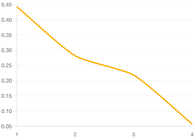
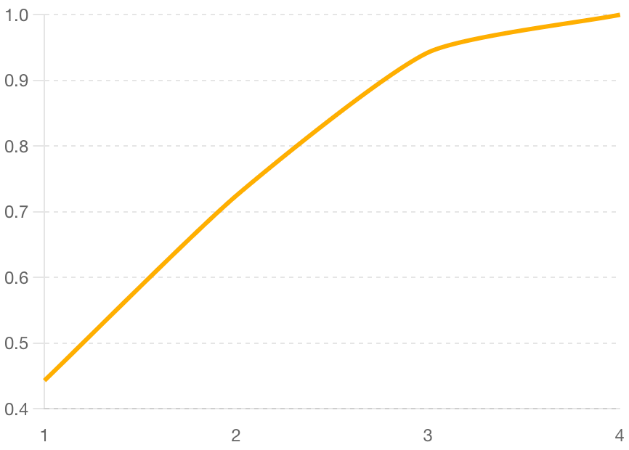
The Scree Plot from Figure 1 helps us determine the number of significant principal components. On the  $$ x$$ -axis, we have the principal components listed in descending order of their variance. The  $$ y$$ -axis shows the explained variance by each component. As we can see from the plot, the first two components explain the majority of the variance. The Cumulative Explained Variance Plot on the right side provides a cumulative sum of the variance explained by each principal component. We can see that first two components capture over 70% of the variance, which indicates that these two components can sufficiently represent the data with minimal loss of information.

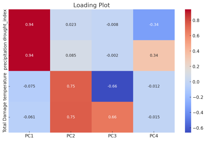
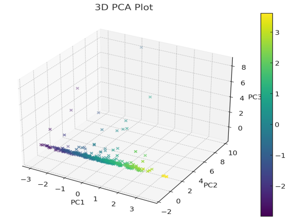
Figure 2 shows the visualized results of PCA. The Loading Plot illustrates the contribution of each original variable to the principal components. Each vector in the plot represents a variable from the original dataset, and its length and direction indicate the variable’s weight in the principal components. We can observe that on the upper left corner of this plot, precipitation and drought index play a significant role in the first principal component. The 3D PCA Plot visualizes the data points projected onto the first three principal components, which allows us to see the clustering and distribution of data points in a reduced three-dimensional space.

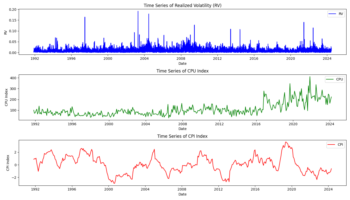
The above steps of building a robust Climate Physical Index (CPI) that captures the essential features of the underlying climate-related variables is pivotal to our later model construction. Our data covers the period from December 1, 1991, to March 28, 2024, the maximum duration allowed by data availability. Figure 3 visually depicts the trends of RV, CPU and CPI.

It is clear that CPU generally showed an upward trend, while CPI experienced larger fluctuations. Table 2 provides their descriptive statistics. It is clear that the raw form of the CPI series is non-stationary. To reject the null hypothesis of the unit root then the CPU exponential sequence can only be at the significance level of 10%. To reduce the risk of false regression, we convert these two predictions by calculating the first-order difference of their logarithmic values. As indicated in Table 2, these transformed series were stationary and therefore used in our empirical analysis in place of the original series.

5.  Empirical results

This section consists of two major parts: in-sample estimation and out-of-sample evaluation. We examine the impact of Climate Policy Uncertainty (CPU) and the Climate Physical Index (CPI) on the volatility of soybean futures prices. The sample data covers the period from November 1, 1991, to March 28, 2024, for in-sample estimation, and from April 1, 2024, onwards for out-of-sample evaluation. The forecasts are conducted using a rolling-window approach.

5.1.  In-sample estimation

The in-sample estimation assesses the efficiency of the GARCH-MIDAS model in capturing the volatility dynamics of soybean futures prices, incorporating daily realized volatility (RV) along with monthly Climate Policy Uncertainty (CPU) and Climate Physical Index (CPI) indices. Four models are considered: RV, RV + CPU, RV + CPI, and RV + CPU + CPI.

Table 3 provides the Maximum Likelihood Estimates (MLE) of the coefficients for these models, with the Bayesian Information Criterion (BIC) determining the maximum lag orders for long-term predictors. The statistically significant ARCH terms ( $$ \alpha $$ ) and GARCH terms ( $$ \beta $$ ) across most models indicate the presence of volatility clustering in soybean futures prices. However, the α and β in the second model are not significant, which means the model lacks predictive power and explanatory power for soybean futures price volatility. The significance of these parameters varies with the inclusion of climate indices, suggesting that external climate factors do impact soybean price volatility.

The MIDAS slope coefficients ( $$ {\theta }_{CPU}$$  and  $$ {\theta }_{CPU}$$ ) are positive in columns (2) and (3) of the Table 3. It shows that these two variables are positively correlated to the long-term volatility of soybean futures price. The significant values of these slope coefficients demonstrate that both CPU and CPI contribute to long-term volatility.

The LLF value gradually increases with the change of the model, the RV model has the lowest value which is 13978.6882, and the RV+CPU+CPI model has the highest LLF value of 14235.3112. This shows that adding CPU and CPI to the model improves the fitness, in other words they provide additional information that affects soybean price fluctuations. This suggests that the inclusion of CPU and CPI in the model improves the fitness of models, as these factors provide additional information that affects soybean price fluctuations. Decreasing in BIC values indicates the complexity of the model increases with the inclusion of CPU and CPI.

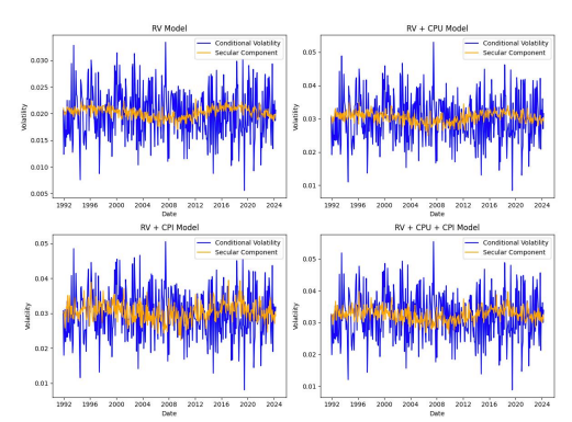
​ Figure 4 shows the total conditional volatility and long-term components obtained from each model. As can be seen from the picture, the calculated total conditional volatility of each model is very similar while the secular components show significant differences. In all models, conditional volatility frequently spikes during periods of market stress or major events affecting soybean futures prices. The RV + CPU and RV + CPI models show higher conditional volatility than the RV model, suggesting that both CPU and CPI are important factors in increasing volatility. The RV + CPU + CPI model exhibits the highest conditional volatility, reflecting the compound effect of CPU and CPI.

The secular component remains relatively smooth in the RV model, indicating a stable long-term trend. However, the RV + CPU + CPI model exhibits the most significant fluctuations in the secular component, underscoring the compounded effects of both types of climate risks on long-term volatility trends.

Overall, the analysis confirms that CPU and CPI have strong tracking and predictive abilities for soybean futures price volatility. However, further analysis is required to evaluate CPU and CPI as long-term volatility predictors in an out-of-sample context.

5.2.  Out-of-sample evaluation

The out-of-sample performance of predictive models is more important than their in-sample performance because market participants are primarily concerned with the model’s ability to forecast future volatility rather than analyze past data [30-32]. This subsection examines whether incorporating climate-related risk factors, namely CPU and CPI, can enhance the predictive ability of soybean futures volatility. We use out-of-sample predictions to directly compare the performances of the extended GARCH-MIDAS models, assessing their effectiveness in forecasting market volatility.

In particular, to evaluate the predictive power of the GARCH-MIDAS model, we apply two loss functions: Mean Squared Error (MSE) and Mean Absolute Error (MAE) [33], as is defined in the following formulae:

$$$ \begin{array}{c}MSE=\frac{1}{n}\sum _{t=1}^n{({{\sigma }_t}^2-{{\widehat{\sigma }}_t}^2)}^2\end{array}$$$(12)

$MAE=1n\sum t=1n\mid \sigma t2-\sigma t2\mid$(13)

where  $$ n$$ ​ equals the total number of days forecasted, and  $$ {\sigma }_t^2$$  and  $$ {{\widehat{\sigma }}_t}^2$$  are the actual and forecast values of the volatility, respectively. Specifically,  $$ {\sigma }_t^2$$  refers to the squared daily return, which serves as a proxy for the actual volatility during the out-of-sample period.  $$ {{\widehat{\sigma }}_t}^2$$  represents the out-of-sample volatility forecast derived from each of the aforementioned models.

Notes:  $$ {MCS}_{MAE}$$  and  $$ {MCS}_{MSE}$$ ​ refer to the p-values of the MCS test, calculated using mean absolute error and mean squared error, respectively. An asterisk (*) represents a p-value > 0.1, indicating that the corresponding model passed the MCS test under the specified loss function. A value of 1.000 indicates the best model of all.

First, we introduce the Model Confidence Set (MCS) to evaluate the forecasts. The p-value reflects the forecasting accuracy of the corresponding model. The model with the largest p-value is considered as the best one [34].

To assess the prediction accuracy over different horizons, we divide the forecasting periods into five lengths. We use 10 days and 30 days to test short-term accuracy, 60 days for mid-term accuracy, and 90 days and 120 days for long-term accuracy. Specifically, we calculated the MSE and MAE for each model.

From the results shown in Table 4, we can conclude that RV has good predictive power, as past volatility tends to affect future volatility, a belief held by technical analysts. Additionally, we observe that CPU has better predictive power than CPI. CPI does not seem to be a good index for forecasting soybean futures volatility. For short-term predictions, CPU holds a slight advantage over CPI, but their performance is almost the same. However, in the long run, CPU shows strong predictive power, becoming almost as accurate as RV. Therefore, the conclusion is that the GARCH-MIDAS model provides appropriate volatility predictions, with better accuracy in the long run. The CPI+RV model consistently underperforms in both MAE and MSE metrics.

When looking at p-values, we find that RV has the best accuracy. The RV+CPU, RV+CPI, and RV+CPU+CPI models all pass the MCS test in the long run, consistent with the MAE and MSE results mentioned above. Among these, CPI appears to have the worst predictive power.

The reason behind this phenomenon may be the time lags associated with climate policy impacts. In other words, investors need time to adjust to the policies. Unlike economic policies, the effects of climate policies are not as immediate or obvious. As a result, CPU affects soybean markets in a way similar to realized volatility. Then the combination of these two variables does not provide sufficient extra information for the forecast.

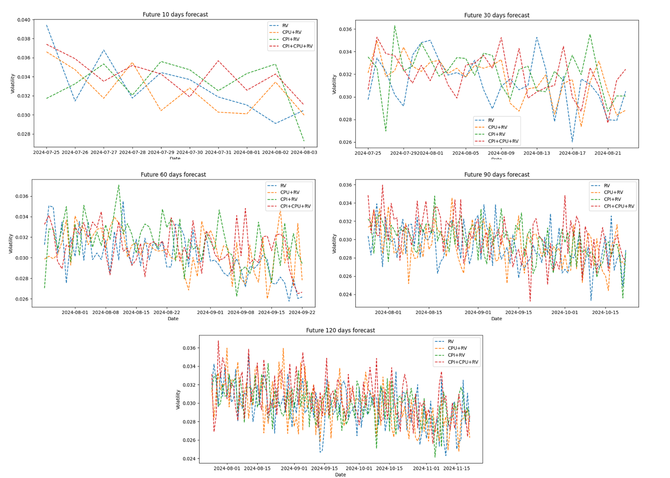
Figure 5 illustrates the forecasted volatility of soybean futures for the next 10, 30, 60, 90, and 120 days. Each subplot corresponds to a different forecast horizon, with predictions generated using a rolling-window approach.

Across all forecast horizons, the models exhibit a consistent trend, but with notable differences in the specific values. Overall, the RV model shows relatively stable volatility predictions across all time periods, while the models incorporating CPU and CPI exhibit more fluctuation. This suggests that Climate Policy Uncertainty (CPU) and Climate Physical Index (CPI) indeed impact the volatility of soybean futures prices.

Specifically, in the 10 - and 30-day short-term forecasts, despite some differences in the volatility forecasts of the four models, the overall trend remains consistent, suggesting that the models are relatively effective at capturing market volatility in the short term. The 60-day medium-term forecasts and the 90 - and 120-day long-term forecasts show that while the volatility forecasts for all four models still show similar trends, the models that incorporate CPU and CPI show greater volatility over time, which may reflect the long-term impact of climate factors on soybean futures prices.

​ Overall, Figure 5 shows that the GARCH-MIDAS model effectively combines high - and low-frequency data to predict volatility in soybean futures prices. Incorporating climate-related variables (CPU and CPI) into the model provides additional information that improves forecast accuracy.

6.  Conclusion

In this paper, we use the GARCH-MIDAS model to forecast the volatility of soybean futures prices. We introduced two climate-related factors—Climate Policy Uncertainty (CPU) and Climate Physical Index (CPI)—as exogenous variables in the GARCH-MIDAS model.

It can be seen from the empirical forecast results that both CPU and CPI will affect the long-term fluctuations of soybean future prices. Higher log-likelihood function (LLF) values and lower Bayesian Information Standard (BIC) scores shown as evidence and testify by adding these variables can improve the predictive power of the model.

In out-of-sample evaluation, we use MCS test to evaluate the predictive power of the models, and then compare each model to another. The empirical results are meant by the longer the prediction accuracy of the model will be higher. The RV model performed best in the short-term forecast period (10 and 30 days). For medium - to long-term forecast periods (60, 90, and 120 days), the combined RV+CPU+CPI model has the best performance. This illustrates that the combined effect of the two climate-related indices significantly improves the forecasted ability of the model in the long-term. The high volatility of the soybean futures market due to uncertainty in climatic policies and climate-related factors is consistent with the empirical findings of Fang et al [35].

In general, the valuation of assets, the pricing of derivatives, risk management, and policymaking all rely on past tracking and future forecasting of volatility [36].Then assessing investment risk requires accurate prediction of asset price changes during the holding period and continuous calculation of their volatility. We also realized the importance of volatility prediction during the research. The results show that climate-related factors, especially CPU index, have a positive and remarkable impact on the soybean futures market. To effectively predict the volatility of soybean futures, traders and policymakers should consider the CPU index when assessing investment risk or conducting derivatives transactions. This conclusion is also very valuable for financial workers.

Acknowledgement

Ziming Wang, Hanqi Hu, Zaihao Hu and Yuxin Jin contributed equally to this work and should be considered co-first authors.

References

[1]. Carleton, T. A., & Hsiang, S. M. (2016). Social and Economic Impacts of Climate. Science, 353(6304), aad9837.
[2]. Guo, K., Li, Y., Zhang, Y., Ji, Q., & Zhao, W. (2023). How Are Climate Risk Shocks Connected to Agricultural Markets? Journal of Commodity Markets, 32, 100367.
[3]. Baker, S. R., Bloom, N., & Davis, S. J. (2016). Measuring Economic Policy Uncertainty. Quarterly Journal of Economics, 131(4), 1593-1636.
[4]. Hong, H., Karolyi, G. A., & Scheinkman, J. A. (2020). Climate Finance. Review of Financial Studies, 33(3), 1043-1071.
[5]. Lee, K., Yang, H., & Huang, Z. (2022). Impact of Climate Policy Uncertainty on Energy Market Volatility. Energy Economics, 100, 105349.
[6]. Nordhaus, W. D. (2019). Climate Change: The Ultimate Challenge for Economics. American Economic Review, 109(6), 1991-2014.
[7]. J in, X., & Cheong, T. (2021). Climate Policy Uncertainty and Agricultural Commodity Prices in Asian Markets. Agricultural Economics, 52(4), 495-507.
[8]. Auffhammer, M. (2018). Climate Physical Risk and Agricultural Commodity Prices. Journal of Environmental Economics and Management, 91, 210-228.
[9]. Matiu, M., Ankerst, D. P., & Menzel, A. (2017). Interactions between Temperature and Drought in Global and Regional Crop Yield Variability during 1961–2014. PLOS ONE, 12(5), e0178339.
[10]. Lobell, D. B., Schlenker, W., & Costa-Roberts, J. (2011). Climate Trends and Global Crop Production Since 1980. Science, 333(6042), 616-620.
[11]. Lesk, C., Rowhani, P., & Ramankutty, N. (2016). Influence of Extreme Weather Disasters on Global Crop Production. Nature, 529(7584), 84-87.
[12]. Schlenker, W., & Roberts, M. J. (2009). Nonlinear Temperature Effects Indicate Severe Damages to U.S. Crop Yields under Climate Change. Proceedings of the National Academy of Sciences, 106(37), 15594-15598.
[13]. Luo, X., Zhang, J., & Ma, C. (2022). Realized Volatility and Its Role in Predictive Models. Journal of Financial Markets, 55, 100605.
[14]. McAleer, M., & Medeiros, M. C. (2008). Realized Volatility: A Review. Econometric Reviews, 27(1-3), 10-45.
[15]. Engle, R. F., Ghysels, E., & Sohn, B. (2013). Stock Market Volatility and Macroeconomic Fundamentals. Review of Economics and Statistics, 95(3), 776-797.
[16]. Raza, N., Shahbaz, M., & Salahuddin, M. (2023). Dynamic Connectedness of Economic Policy Uncertainty and Financial Stress: Evidence from GARCH-MIDAS Models. Journal of Financial Stability, 60, 100921.
[17]. Salisu, A. A., Ndako, U. B., & Oloko, T. F. (2022). Forecasting Stock Market Volatility with Macroeconomic Variables: Evidence from GARCH-MIDAS Models. International Review of Financial Analysis, 82, 101933.
[18]. Fang, L., Chen, B., & Li, Z. (2020). The Impact of Economic Policy Uncertainty on Stock Market Volatility: Evidence from China. Finance Research Letters, 32, 101304.
[19]. Fang, T., Lee, T. H., & Su, Z. (2020). Predicting the long-term stock market volatility: A GARCH-MIDAS model with variable selection. Journal of Empirical Finance, 58, 36-49.
[20]. Ghysels, E., Sinko, A., & Valkanov, R. (2007). MIDAS regressions: Further results and new directions. Econometric reviews, 26(1), 53-90.
[21]. Luo, X., Tao, Y., & Zou, K. (2022). A new measure of realized volatility: Inertial and reverse realized semivariance. Finance Research Letters, 47, 102658.
[22]. Chuang, O. C., & Yang, C. (2022). Identifying the determinants of crude oil market volatility by the multivariate GARCH-MIDAS model. Energies, 15(8), 2945.
[23]. Dai, P. F., Xiong, X., Zhang, J., & Zhou, W. X. (2022). The role of global economic policy uncertainty in predicting crude oil futures volatility: Evidence from a two-factor GARCH-MIDAS model. Resources Policy, 78, 102849.
[24]. Lang, Q., Lu, X., Ma, F., & Huang, D. (2022). Oil futures volatility predictability: Evidence based on Twitter-based uncertainty. Finance Research Letters, 47, 102536.
[25]. Gavriilidis, K., 2021. Measuring Climate Policy Uncertainty. Available at SSRN: https: //ssrn.com/abstract=3847388.
[26]. Malhi, Gurdeep Singh, Manpreet Kaur, and Prashant Kaushik. "Impact of climate change on agriculture and its mitigation strategies: A review." Sustainability 13.3 (2021): 1318.
[27]. Hatfield, J. L., Boote, K. J., Kimball, B. A., Ziska, L. H., Izaurralde, R. C., Ort, D., ... & Wolfe, D. (2011). Climate impacts on agriculture: implications for crop production. Agronomy journal, 103(2), 351-370.
[28]. Mahato, A. (2014). Climate change and its impact on agriculture. International journal of scientific and research publications, 4(4), 1-6.
[29]. Greenacre, Michael, et al. "Principal component analysis." Nature Reviews Methods Primers 2.1 (2022): 100.
[30]. Ma, Y. R., Ji, Q., & Pan, J. (2019). Oil financialization and volatility forecast: Evidence from multidimensional predictors. Journal of Forecasting, 38(6), 564–581.
[31]. Ma, F., Liao, Y., Zhang, Y., & Cao, Y. (2019). Harnessing jump component for crude oil volatility forecasting in the presence of extreme shocks. Journal of Empirical Finance, 52, 40–55.
[32]. Wang, L., Ma, F., Liu, J., & Yang, L. (2020). Forecasting stock price volatility: New evidence from the GARCH-MIDAS model. International Journal of Forecasting, 36(2), 684-694.
[33]. Chicco, D., Warrens, M. J., & Jurman, G. (2021). The coefficient of determination R-squared is more informative than SMAPE, MAE, MAPE, MSE and RMSE in regression analysis evaluation. Peerj computer science, 7, e623.
[34]. Hansen, P. R., Lunde, A., & Nason, J. M. (2011). The model confidence set. Econometrica, 79(2), 453-497.
[35]. Fang, L., Chen, B., Yu, H., & Qian, Y. (2018). The importance of global economic policy uncertainty in predicting gold futures market volatility: A GARCH‐MIDAS approach. Journal of Futures Markets, 38(3), 413-422.
[36]. Asgharian, H., Hou, A. J., & Javed, F. (2013). The importance of the macroeconomic variables in forecasting stock return variance: A GARCH‐MIDAS approach. Journal of Forecasting, 32(7), 600-612.
Cite this article
Wang,Z.;Hu,H.;Hu,Z.;Jin,Y. (2025). Forecasting Soybean Futures Volatility: The Impact of Climate -Related Indices Using GARCH-MIDAS Model. Advances in Economics, Management and Political Sciences,198,43-56.
Data availability
The datasets used and/or analyzed during the current study will be available from the authors upon reasonable request.
Disclaimer/Publisher's Note
The statements, opinions and data contained in all publications are solely those of the individual author(s) and contributor(s) and not of EWA Publishing and/or the editor(s). EWA Publishing and/or the editor(s) disclaim responsibility for any injury to people or property resulting from any ideas, methods, instructions or products referred to in the content.
About volume
Volume title: Proceedings of the 3rd International Conference on Financial Technology and Business Analysis
© 2024 by the author(s). Licensee EWA Publishing, Oxford, UK. This article is an open access article distributed under the terms and
conditions of the Creative Commons Attribution (CC BY) license. Authors who
publish this series agree to the following terms:
1. Authors retain copyright and grant the series right of first publication with the work simultaneously licensed under a Creative Commons
Attribution License that allows others to share the work with an acknowledgment of the work's authorship and initial publication in this
series.
2. Authors are able to enter into separate, additional contractual arrangements for the non-exclusive distribution of the series's published
version of the work (e.g., post it to an institutional repository or publish it in a book), with an acknowledgment of its initial
publication in this series.
3. Authors are permitted and encouraged to post their work online (e.g., in institutional repositories or on their website) prior to and
during the submission process, as it can lead to productive exchanges, as well as earlier and greater citation of published work (See
Open access policy for details).