1.  Introduction

As one of the core elements of the economic market, stocks closely reflect the overall operation trend of the macro-economy. Especially in the domestic stock market, the stock fluctuations of some large financial groups reflect the state of the national economy to a certain extent. Therefore, both investors and managers are paying close attention to the trend of stock prices, and stock price prediction has become a popular financial study topic.

In recent years, time series analysis and machine learning have received extensive attention from researchers in stock price prediction. Cui used the ARIMA, ARCH and GARCH models in time series analysis to study stock returns and found that the ARIMA model had the best fitting effect [1]. Huang explained the modeling process and model evaluation of the ARIMA model in detail, pointing out that the ARIMA model is appropriate for short-term predictions, but further research is needed for long-term prediction [2]. Many researchers have begun to combine ARIMA models with machine learning models. The prediction effects of Fu's ARIMA-RF combined model [3]and Guan's ARIMA-RNN hybrid model were better than those of a single model, which effectively improved the prediction accuracy [4]. Xiao forecasted stock values using the LSTM and ARIMA models and found that ARIMA had a good short-term prediction effect, while LSTM was more effective in predicting all stock prices, but no model combination was performed [5]. Gu successfully increased the model's prediction accuracy after mixing by feeding the ARIMA model's prediction error into LSTM [6]. Due to the large volatility of stock prices, some researchers also use gray models to predict them. Tian et al. proposed a similar gray model based on the entanglement theory, which effectively improved the prediction accuracy of oscillation sequences [7]. On this basis, Guo et al. established the ARIMA-GM multivariate regression model based on the grey theory and optimized the fitting effect [8].

The above studies mostly use a single method to select ARIMA model parameters. This paper uses a variety of methods to select parameters and compare them, then establishes a residual-corrected GM (2,1) model, mixes the GM model with the ARIMA model by weighted average, and forecasts stock prices using it, and compares the prediction results with those of the LSTM model.

2.  Data and model methods

2.1.  Source and description of data

The source of the data is the AKShare data interface. Pyhton crawled the monthly stock prices of Ping An of China from January 2016 to December 2024 on AKShare as the research object. The data includes date, opening price, closing price, top price, bottom price, number of traded stocks and transaction amount, a total of 108 data.

2.2.  Selection and description of indicators

This paper only uses closing prices for empirical research. The closing price is the price at which a stock was last traded at the end of a trading day. Investors closely monitor it, which might show the market's supply and demand balance at the end of the trading day. When evaluating the model performance, this paper contrasts meaning absolute error (MAE), mean relative error (MSE), and root mean squared error (RMSE), with the priority of MSE>RMSE>MAE. The calculation formula for the three indicators are as follows:

$$$ MSE=\frac{1}{n}\sum _{i=1}^n{\left(y_i-{\widehat{y}}_i\right)}^2$$$(1)

$$$ RMSE=\sqrt{\frac{1}{n}\sum _{i=1}^n{\left(y_i-{\widehat{y}}_i\right)}^2}$$$(2)

$$$ MAE=\frac{1}{n}\sum _{i=1}^n\left|y_i-{\widehat{y}}_i\right|$$$(3)

The sample size is n, and the actual value is  $$ y_i$$ , whereas the anticipated value is  $$ {\widehat{y}}_i$$ ,

2.3.  Methods introduction

2.3.1.  ARIMA model

ARIMA model is commonly used in time series analysis. It is made up of three parts: AR (autoregressive model), I (difference process) and MA (moving average model). The time series' historical values are used by the AR part to forecast the present value. The I part transforms the non-stationary series into a stationary series by performing differential processing on the initial data. The MA part uses the past prediction errors to correct the prediction [9]. The ARIMA model has three parameters. 'p’ represents the autoregressive order, 'd’ represents the difference order, and 'q’ represents the moving average order. The ARIMA(p, d, q) may be stated mathematically as follows:

$$$ AR:y_t=c+{\varnothing }_1{y}_{t-1}+{\varnothing }_2{y}_{t-2}+\cdots +{\varnothing }_p{y}_{t-p}+{ϵ}_t$$$(4)

$$$ I:{∆}^d{y}_t={∆}^{d-1}{y}_t-{∆}^{d-1}{y}_{t-1}$$$(5)

$$$ MA:y_t=c+{ϵ}_t+{\theta }_1{ϵ}_{t-1}+{\theta }_2{ϵ}_{t-2}+\cdots +{\theta }_q{ϵ}_{t-q}$$$(6)

$$$ ARIMA:{∆}^d{y}_t=c+{\varnothing }_1{∆}^d{y}_{t-1}+\cdots +{\varnothing }_p{∆}^d{y}_{t-p}+{ϵ}_t+{\theta }_1{ϵ}_{t-1}+\cdots +{\theta }_q{ϵ}_{t-q}$$$(7)

In which  $$ t$$  is the current time point,  $$ y_t$$  is the value at the current time point,  $$ {\mathrm{\varnothing }}_i$$  is the autoregressive coefficient $$ \left(i=1,2,\cdots ,p\right)$$ ,  $$ {\theta }_i$$  is the moving average coefficient $$ (i=1,2,\cdots ,q)$$ ,  $$ {ϵ}_t$$  represents the error at the current time point, whereas  $$ c$$  is the time series' long-term mean.

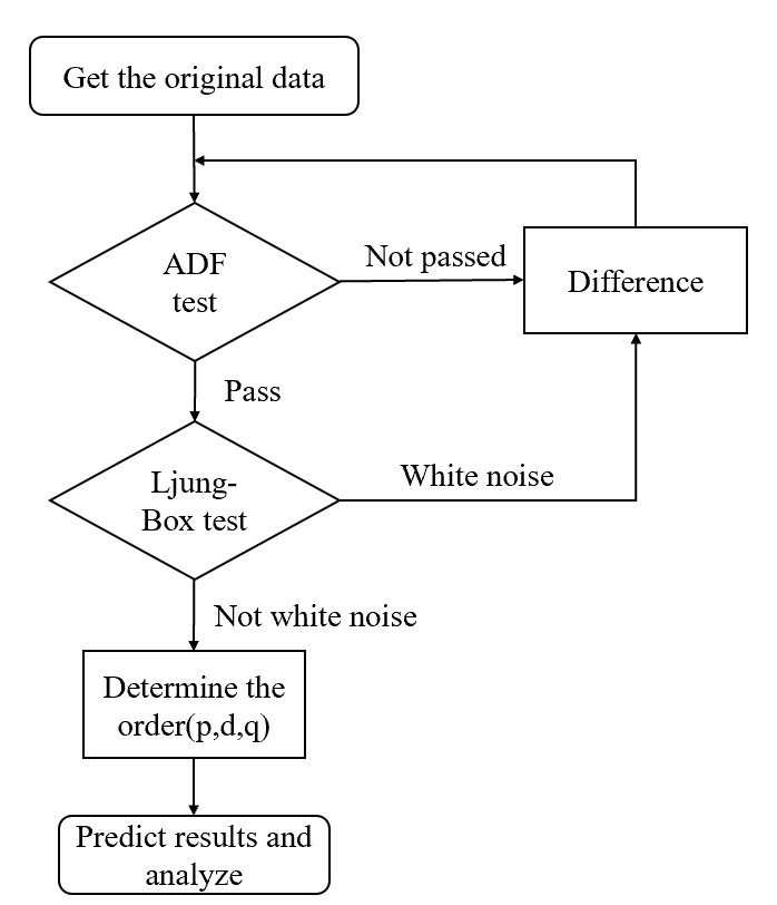
The modeling procedure for the ARIMA model involves stationarity test (divided into Augmented Dickey-Fuller test and Ljung-Box test), model order determination, model prediction and other parts. Figure 1 shows the exact flow chart:

2.3.2.  Grey Theory Model: GM (2,1)

Famous professor Deng Julong proposed the grey system hypothesis, and it is used to deal with systems with small samples, strong uncertainty, and incomplete information. The simplest model in grey system theory, GM (1,1), is frequently employed for time series data. GM (2,1) introduces a second-order differential equation based on GM (1,1), which can better handle nonlinear and volatile data. The modeling process is as follows.

Assume the original time series is:

$$$ X^{\left(0\right)}=\left\{x^{\left(0\right)}\left(1\right),x^{\left(0\right)}\left(2\right),\cdots ,x^{\left(0\right)}\left(n\right)\right\}$$$(8)

In which  $$ x^{\left(0\right)}\left(k\right)$$  represents the observed value at the kth time point. Then the original sequence is accumulated once to obtain the cumulative sequence  $$ X^{\left(1\right)}$$ :

$$$ x^{\left(1\right)}\left(k\right)=\sum _{i=1}^k{x}^{\left(0\right)}\left(i\right),k=\mathrm{1,2},\cdots ,n$$$(9)

According to the cumulative sequence, the second-order differential equation is obtained:

$$$ \frac{d^2{x}^{\left(1\right)}}{d{t}^2}+a_1\frac{d{x}^{\left(1\right)}}{dt}+a_2{x}^{\left(1\right)}=b$$$(10)

In which  $$ a_1$$ , $$ a_2$$  and  $$ b$$ are all parameters to be estimated, and the equation is solved using the least squares method:

$$$ \begin{array}{c}\widehat{a}={\left[\begin{array}{ccc}{a}_1& a_2& b\end{array}\right]}^T={\left(B^{T}B\right)}^{-1}{B}^{T}Y\\ Observation Matrix:Y={\left[\begin{array}{cccc}{x}^{\left(0\right)}\left(2\right)& x^{\left(0\right)}\left(3\right)& \cdots & x^{\left(0\right)}\left(n\right)\end{array}\right]}^T\\ Coefficient Matrix:B=\left[\begin{array}{ccc}-z^{\left(1\right)}\left(2\right)& -x^{\left(1\right)}\left(2\right)& 1\\ -z^{\left(1\right)}\left(3\right)& -x^{\left(1\right)}\left(3\right)& 1\\ ⋮& ⋮& ⋮\\ {-z}^{\left(1\right)}\left(n\right)& -x^{\left(1\right)}\left(n\right)& 1\end{array}\right]\end{array}$$$(11)

The equation's solution is the expected value of the cumulative sequence  $$ {\widehat{x}}^{\left(1\right)}\left(k\right)$$ , which is then subtracted to get the anticipated value of the original sequence  $$ {\widehat{x}}^{\left(0\right)}\left(k\right)$$ :

$$$ {\widehat{x}}^{\left(0\right)}\left(k\right)={\widehat{x}}^{\left(1\right)}\left(k\right)-{\widehat{x}}^{\left(1\right)}\left(k-1\right),k=\mathrm{2,3},\cdots ,n$$$(12)

2.3.3.  ARIMA-GM hybrid model

The mixed mode of the model is weighted average mixing, that is, the predicted value of the mixed model is expressed as:

$$$ {\widehat{y}}_t=w{{\widehat{y}}_t}^{ARIMA}+\left(1-w\right){{\widehat{y}}_t}^{GM\left(\mathrm{2,1}\right)}$$$(13)

In which  $$ w$$  is the weight coefficient, which is determined by grid search method, optimization algorithm, cross validation method and Bayesian optimization method in this paper.

To increase the hybrid model's predictive accuracy, this paper uses the moving average approach to smooth the prediction outcomes of the GM (2,1). Here's the specific method:

$$$ e\left(k\right)=x^{\left(0\right)}\left(k\right)-{\widehat{x}}^{\left(0\right)}\left(k\right)$$$(14)

$$$ e=\left[e\left(1\right),e\left(2\right),\cdots ,e\left(n\right)\right]$$$(15)

In which  $$ e\left(k\right)$$  is the residual at the kth time point. Then the residual sequence e is moved averaged to obtain the smoothed residual sequence:

$$$ e_{smootℎ}\left(k\right)=\frac{e\left(k\right)+e\left(k-1\right)+\cdots +e\left(k-ℎ+1\right)}{ℎ}$$$(16)

In which  $$ ℎ$$  is the number of time points of the moving average. Add the smoothed residual to the original forecast value to get the revised forecast value:

$$$ {{\widehat{x}}^{\left(0\right)}}_{corrected}\left(k\right)={\widehat{x}}^{\left(0\right)}\left(k\right)+e_{smootℎ}\left(k\right)$$$(17)

2.3.4.  LSTM model

Long Short-Term Memory(LSTM) is a type of improved Recurrent Neural Networks. Long-term dependencies are hard for the model to learn with typical RNNs since the gradient either decays or climbs exponentially as the number of time steps increases during training. LSTM adds memory units and gating mechanisms, this successfully overcomes the gradient disappearing and gradient bursting concerns of RNN while processing lengthy sequence data. [10]. LSTM working diagram is given in Figure 2:

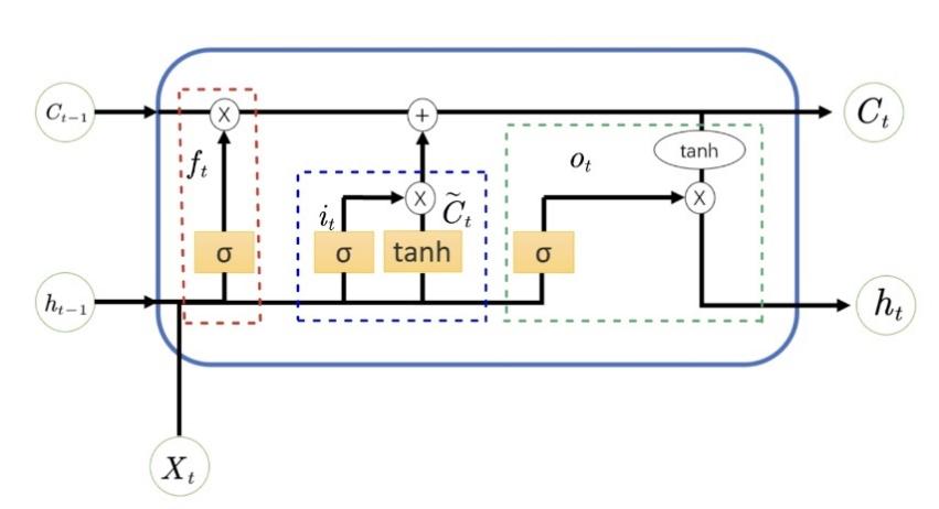
In figure 2,  $$ \left\{X_1,X_2,\cdots ,X_t\right\}$$  is the data input,  $$ \left\{C_1,C_2,\cdots ,C_t\right\}$$  is the memory cell state, and  $$ \left\{H_1,H_2,\cdots ,H_t\right\}$$  is the hidden state.

Forget Gate  $$ f_t$$ : It determines which information is discarded. The hidden state  $$ H_{t-1}$$  of the previous time step and the input  $$ X_t$$  of the current time step are concatenated into a vector, which is then linearly transformed and input into the Sigmoid activation function to obtain a number in the interval [0,1]. If  $$ f_t=0$$ , the information in the memory cell is completely retained; if  $$ f_t=1$$ , it is completely retained; if  $$ {0<f}_t<1$$ , it is partially retained. The specific expression is as follows:

$$$ f_t=\sigma \left(W_f\bullet \left[H_{t-1},X_t\right]+b_f\right)$$$(18)

In which  $$ W_f$$  is the weight matrix of the forget gate,  $$ b_f$$  represented the bias term, and  $$ \sigma $$  is the activation function.

Input Gate  $$ i_t$$ : It determines which new information is stored in the memory cell. The Sigmoid activation function is used to output a number between [0,1], indicating the retention ratio of the new information, in addition, the tanh activation function is employed to construct the candidate memory cell state simultaneously. The output result is the sum of the forget gate's product with the memory cell state at the previous time step, as well as the new information added under the control of the input gate. The specific expression is as follows:

$$$ i_t=\sigma \left(W_i\bullet \left[H_{t-1},X_t\right]+b_i\right)$$$(19)

$$$ {\tilde{C}}_t=\tanh \left(W_C\bullet \left[H_{t-1},X_t\right]+b_C\right)$$$(20)

$$$ C_t=f_t\bullet C_{t-1}+i_t\bullet {\tilde{C}}_t$$$(21)

In which  $$ {\tilde{C}}_t$$  denotes the candidate memory cell, whereas  $$ W_i$$  and  $$ W_C$$  represent the weight matrices for the input gate and candidate memory unit respectively,  $$ b_i$$  and  $$ b_C$$  are both bias terms.

Output Gate  $$ o_t$$ : It determines what data the memory cell  $$ C_t$$  sends to the hidden state  $$ H_t$$ . After compressing the memory cell state to [-1,1] using the tanh activation function and creating a number in the [0,1] interval with the Sigmoid activation function, the output is the outcome of the two previously stated components. Here are the precise expressions:

$$$ o_t=\sigma \left(W_o\bullet \left[H_{t-1},X_t\right]+b_o\right)$$$(22)

$$$ H_t=o_t\bullet \tanh \left(C_t\right)$$$(23)

 $$ W_o$$  is the weight matrix of the output gate, while  $$ b_o$$  is the bias term.

3.  Empirical analysis

This paper's models employ Ping An of China’s data from January 2016 to November 2023 is used as the training set, and the remaining data from December 2023 to December 2024 is used as the test set.

3.1.  ARIMA model analysis

3.1.1.  Stationarity test

The original data is examined for stationarity. This paper separates it into two rounds: ADF test and Ljung-Box test. Only when both sets of tests pass can the sequence be called stationary. The test statistics are all below the critical thresholds of 1%, 5%, and 10%, and the p-value is less than the significance level of 0.05, which means that the test has passed. The ADF test results in Table 1. show that the original sequence fails, while the first-order difference sequence and the second-order difference sequence both pass. For the Ljung-Box test, the p-value less than the significance level of 0.05 is considered to have passed the test. The results are shown in Table 2.

Through the above two rounds of tests, it can be considered that the second-order difference sequence is a stationary sequence.

3.1.2.  Parameter determination

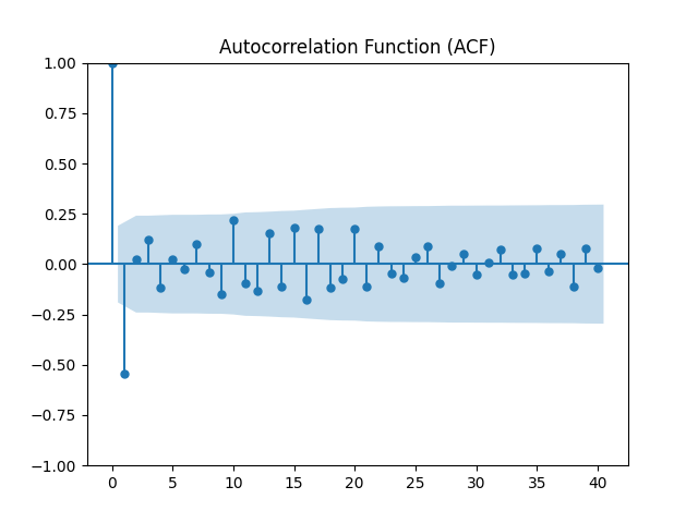
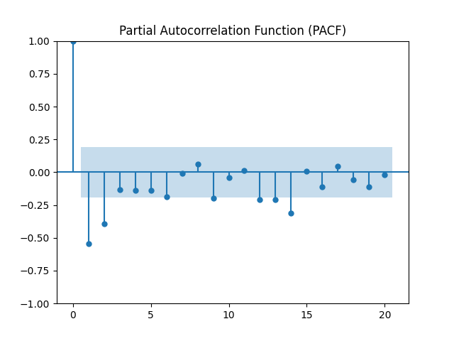
The result of the stationarity test shows that the difference order is d=2. To determine p and q, this paper uses four methods: autocorrelation figure (ACF) and partial autocorrelation figure (PACF), AIC minimum criterion, BIC minimum criterion and cross-validation technique are used to find the best parameters by comparing their MSE, RMSE, and MAE values. Figures 3 and 4 illustrate the ACF and the PACF. It can be seen from the two figures that the ACF is shortened at order=1, whereas the PACF is truncated at order=2, so p=2, q=1. The final parameter results are shown in Table 3.

After comprehensive comparison, ARIMA (2,2,4) was finally selected as the optimal model.

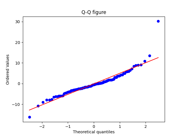
3.1.3.  Model checking

This paper uses QQ graph to test the model, as shown in Figure 5. After observing the QQ graph, it is found that most of the data points are near the straight line. It can be considered that the residuals conform to the normal distribution characteristics and the model can make effective predictions.

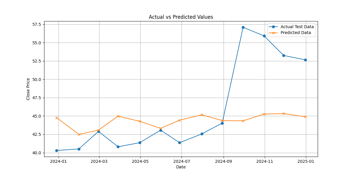
3.1.4.  Prediction results

The prediction results of the ARIMA (2,2,4) model are shown in Figure 6.

3.2.  GM (2,1) model analysis

3.2.1.  Prediction results

According to the formula mentioned above, the number of time points for moving average is selected as h=3, Using Python to calculate the modified GM (2,1) model parameters, and solve for  $$ a_1=-0.025$$ ,  $$ a_2=0.006$$ ,  $$ b=36.189$$ . Substituting the parameters into the second-order differential equation, continue to use Python to solve and predict, and obtain the results shown in Figure 7.

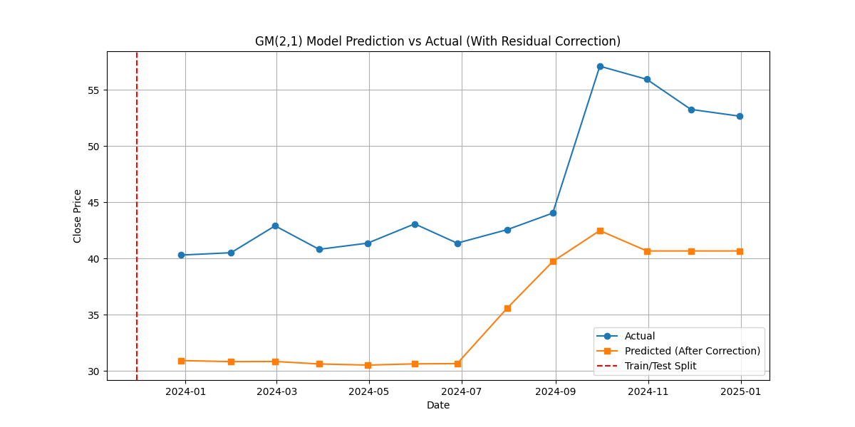
3.2.2.  Model evaluation

The model was subjected to posterior difference test and association test. The posterior difference ratio  $$ C=0.214<0.35$$ , the small error probability  $$ p=1>0.95$$ ,and the correlation is 0.67, close to 1. The above shows that the model has good prediction accuracy.

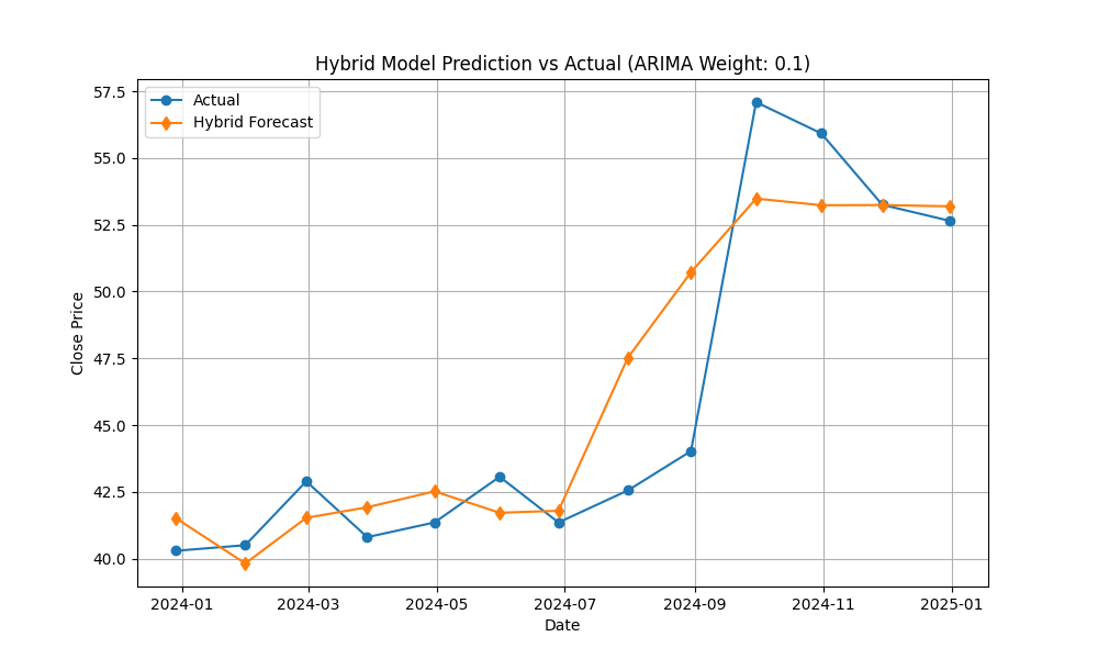
3.3.  ARIMA (2,2,4)-GM (2,1) hybrid model analysis

This paper proposes an ARIMA-GM hybrid model based on the ARIMA model and the GM model, and the hybrid method is weighted average hybrid. The optimal weight is selected according to the above formula (18), and the results are shown in Table 4.

The above table shows that 0.11 is the optimal weight that may be obtained by adopting the minimum MSE strategy:

$$$ {\widehat{y}}_t=0.11{{\widehat{y}}_t}^{ARIMA}+0.89{{\widehat{y}}_t}^{GM\left(\mathrm{2,1}\right)}$$$(24)

Results of the forecast are displayed in Figure 8.

3.4.  LSTM model analysis

3.4.1.  Data processing

In order to speed up the training process and improve model performance, the original data is generally not directly input into the LSTM model, but is normalized first. This paper uses the Min-Max normalization method to scale the data to the interval [0,1]. The specific formula is as follows:

$$$ X_{norm}=\frac{X-X_{min}}{X_{max}-X_{min}}$$$(25)

Where  $$ X$$  is the original data,  $$ X_{max}$$  is the maximum value, and  $$ X_{min}$$  is the minimum value.

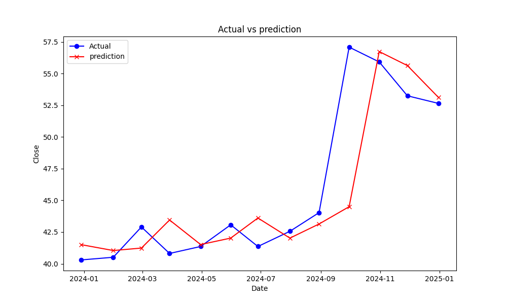
3.4.2.  Prediction results

The LSTM model in this paper contains 2 hidden layers and 1 fully connected layer. Each hidden layer has 50 neurons, whereas the fully connected layer has 25 neurons. MSE is the loss function, whereas Adam is the optimization function. Each training uses 12 samples and is trained 100 times. The final prediction results are shown in Figure 9.

3.5.  Model comparison

The model performance comparison of ARIMA (2,2,4), GM (2,1), ARIMA-GM hybrid model and LSTM model is shown in Table 5.

Table 5 demonstrates that the ARIMA and GM models' prediction results are inferior to the LSTM model, while the ARIMA-GM model after weighted mixing outperforms the LSTM model.

4.  Conclusion

This paper selects the historical closing price of Ping An of China as a time series, and constructs ARIMA, GM, LSTM and ARIMA-GM hybrid model to predict future stock prices. The empirical results reveal that the hybrid model's prediction impact is superior to both the LSTM model and the individual ARIMA and GM models. The hybrid model's ARIMA model can capture linear data features, while the GM model can catch nonlinear ones, which explains this. The accuracy of the predictions can be increased by combining the two. Future stock price predictions can be made more accurate by increasing the model's prediction accuracy., better help investors avoid risks and increase returns, and also help managers balance the market and promote market stability.

At the same time, the hybrid model described in this paper also has shortcomings. This paper's data set is divided in a predetermined way. This fixed division method may not adapt to the dynamic changes of the data, especially when the data has obvious trends or seasonality. In subsequent research, we can try to use rolling forecast or cross-validation methods to further optimize the performance of the model.

References

[1]. Yupeng Cui. Application of Time Series Analysis in Stock Returns——Based on ARIMA and ARCH Models. FUJIAN ZHILIANG GUANLI, 2020(2): 184, 183.
[2]. Mengting Huang. An Empirical Study on Stock Price Prediction Based on ARIMA Model. NEI JIANG Science & Technology, 2023, 44(03): 61-62.
[3]. Fu Wenzhi. Research on Stock Price Prediction based on ARIMA-RF Combination Model. Scientific and Technological Innovation, 2023, (08): 40-43.
[4]. GUAN Xueying. Stock price prediction based on ARIMA - RNN hybrid mode. Journal of Harbin University of Commerce (Natural Sciences Edition).2024, 40(02): 250-256.
[5]. Jie Xiao. Research on Stock Price Prediction Based on ARIMA and LSTM Neural Network—Taking Citic Securities (600030) as an Example. E-Commerce Letters, 2024, 13(4): 11.
[6]. Zhenhong Gu. Stock Price Prediction Based on ARIMA-LSTM—A Case Study of Kweichow Moutai. E-Commerce Letters, 2024, 13(4): 10.
[7]. Tian Hongli, Li Chengqun, Yan Huiqiang. Research and application of prediction method based on entanglement theory and similar grey model in prediction of stock price inflection point. Application Research of Computers, 2020, 37(06): 1666-1669+1678.
[8]. GUO Gaiwen, WANG Shihan. Stock Price Prediction Based on Grey Theory and ARIMA Mode. Journal of Henan Institute of Education (Natural Science Edition), 2023, 32(02): 22-27.
[9]. Mohd Faizan Rizvi1, Shivang Sahu2, Dr. Sadhana Rana. ARIMA Model Time Series Forecasting. International Journal for Research in Applied Science and Engineering Technology. 2024, 12(5), 3782-3785.
[10]. Wang Fei. Research progress and application of LSTM recurrent neural network. Heilongjiang University, 2021.
Cite this article
Huang,X. (2025). Stock Price Prediction Based on ARIMA-GM Hybrid and LSTM Model. Advances in Economics, Management and Political Sciences,205,22-35.
Data availability
The datasets used and/or analyzed during the current study will be available from the authors upon reasonable request.
Disclaimer/Publisher's Note
The statements, opinions and data contained in all publications are solely those of the individual author(s) and contributor(s) and not of EWA Publishing and/or the editor(s). EWA Publishing and/or the editor(s) disclaim responsibility for any injury to people or property resulting from any ideas, methods, instructions or products referred to in the content.
About volume
Volume title: Proceedings of ICEMGD 2025 Symposium: The 4th International Conference on Applied Economics and Policy Studies
© 2024 by the author(s). Licensee EWA Publishing, Oxford, UK. This article is an open access article distributed under the terms and
conditions of the Creative Commons Attribution (CC BY) license. Authors who
publish this series agree to the following terms:
1. Authors retain copyright and grant the series right of first publication with the work simultaneously licensed under a Creative Commons
Attribution License that allows others to share the work with an acknowledgment of the work's authorship and initial publication in this
series.
2. Authors are able to enter into separate, additional contractual arrangements for the non-exclusive distribution of the series's published
version of the work (e.g., post it to an institutional repository or publish it in a book), with an acknowledgment of its initial
publication in this series.
3. Authors are permitted and encouraged to post their work online (e.g., in institutional repositories or on their website) prior to and
during the submission process, as it can lead to productive exchanges, as well as earlier and greater citation of published work (See
Open access policy for details).