1. Introduction

The financial and stock markets are characterized by high volatility and unpredictability, posing significant challenges for investors in forecasting stock trends and prices. Precise forecasts are essential for enhancing profits and reducing risks, especially in both short-term trading and long-term investment plans. However, market volatility, influenced by economic, political, and psychological elements, continues to pose challenges to decision-making, even with improvements in analytical techniques. This underscores the necessity of developing robust predictive models to enhance market analysis. The ability to estimate future stock values with precision offers substantial economic benefits, making stock market forecasting a critical area of research for both academia and practitioners.

While numerous studies have explored stock market prediction, many traditional models fail to fully account for non-linear trends and external uncertainties, limiting their accuracy. The Autoregressive Integrated Moving Average (ARIMA) model. The ARIMA model includes autoregressive (AR) model, moving average (MA) model, and seasonal autoregressive integrated moving average (SARIMA) model, widely used in time-series forecasting [1]. More precisely, forecasting in the realm of time series entails leveraging a particular model to predict forthcoming values of a variable that encapsulates aspects of a phenomenon, grounded in extant historical data [2]. When analyzing specific stocks of fast-growing consumer brands like Pop Mart, they are still not fully utilized. This study addresses this gap by applying the ARIMA model to predict Pop Mart’s stock trends, combining theoretical rigor with practical relevance. The objectives include elucidating the ARIMA framework, detailing its construction and validation steps, and demonstrating its efficacy through a case study. Identifying the best model among the various combinations of non-seasonal and seasonal orders is crucial for achieving good forecasting performance with ARIMA models, given the rich variation they provide [3].

The paper is structured as follows: First, it provides a comprehensive overview of the ARIMA model and its applicability to stock market analysis. Next, it outlines the methodology, including data preprocessing, model selection, and accuracy verification. Finally, a case study of Pop Mart’s stock is presented to validate the model’s predictive performance, followed by conclusions and implications for investors.

2. Time series model

The order of integration, which indicates the number of differencing operations needed to achieve stationarity in a time series, is what the term "integrated" refers to [4]. Within this framework, the forthcoming value in a time series data set  $$ X_t$$  is delineated mathematically by

$$$ \begin{array}{c}\left(1-{\sum }_{i=1}^p{\mathrm{\phi }}_i{B}^i\right){\left(1-B\right)}^d{X}_t=\left(1+{\sum }_{j=1}^q{\mathrm{\theta }}_j{B}^j\right){\mathrm{ϵ}}_t\end{array}$$$(1)

where  $$ B$$  is the lag operator,  $$ p$$  and  $$ q$$  are the parameters of the autoregressive and moving average ARIMA (p, d, q), with d representing the order of integration.

3. Model building

3.1. Data pretreatment

Prior to constructing the model, it is essential to assess whether the data is white noise and whether it exhibits stability. If the data is identified as a white noise series, it holds little significance for the research. Conversely, if the data is unstable, the final results may significantly deviate from the actual situation. To address this, the data must be differenced until it achieves stability [5]. Following differencing, the new dataset will undergo the Augmented Dickey-Fuller (ADF) test to confirm its stability. Should the ADF test yield a p-value greater than 0.05, indicating that the data remains unstable, further differencing and retesting are required. The parameter d in the integrated (I) component represents the number of differencing operations performed. Additionally, the Box-Ljung test will be employed to check for white noise. If the test result is less than 0.05, the null hypothesis will be rejected, suggesting that the time series is not white noise. Only after these checks are passed can the study proceed; otherwise, the time series is deemed unsuitable for analysis.

3.2. Estimation of model parameters

The initial estimation of the potential values for the parameters p and q in an ARIMA model can be done using the Autocorrelation Function (ACF) and Partial Autocorrelation Function (PACF). p is used for Autoregressive, d is used for to make the time series data stationary, q is used for Moving Average, ARIMA is able to forecast stationary time series data [6]. For a more precise determination, the Akaike Information Criterion (AIC) and Bayesian Information Criterion (BIC) are employed. The goal is to choose the model with the smallest AIC or BIC value. After determining the values for p, d, and q, the model's parameters will be estimated using Ordinary Least Squares (OLS) and Maximum Likelihood Estimation (MLE) methods.

3.3. Model testing and predicting

Once the predictive model has been constructed, it is imperative to evaluate the residuals through a white noise test and an overfitting test. These assessments are crucial to verify the model's efficacy and to confirm that the residuals adhere to white noise characteristics, which are essential for reliable forecasting. Additionally, upon finalizing the predictive model, the Mean Absolute Percentage Error (MAPE) metric will be implemented to assess its predictive accuracy.

4. Application

4.1. Target companies and time series charts

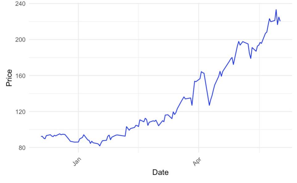
The article will analyze the publicly available stock price data of Pop Mart, spanning the period from December 2024 to May 2025. Utilizing R software, a time series plot of the daily opening prices for POP MART will be generated. Upon examination of the figure (referred to as Figure 1), it is evident that the data exhibits minor fluctuations and predominantly follows a stable upward trajectory.

4.2. Stability testing and differentiation

In order to achieve stationarity in the original time series data, differentiation is applied, followed by the ADF test to ascertain the smoothness of the resulting series. The data satisfies the stationarity condition, as evidenced by an ADF test p-value falling below the threshold of 0.05 after the application of two differencing operations. Concurrently, the white noise test produces a p-value that is less than 0.05, signifying that the data does not conform to a white noise process. This finding validates the non-white noise characteristic of the series, thereby justifying the continuation of the analysis.

4.3. Model building

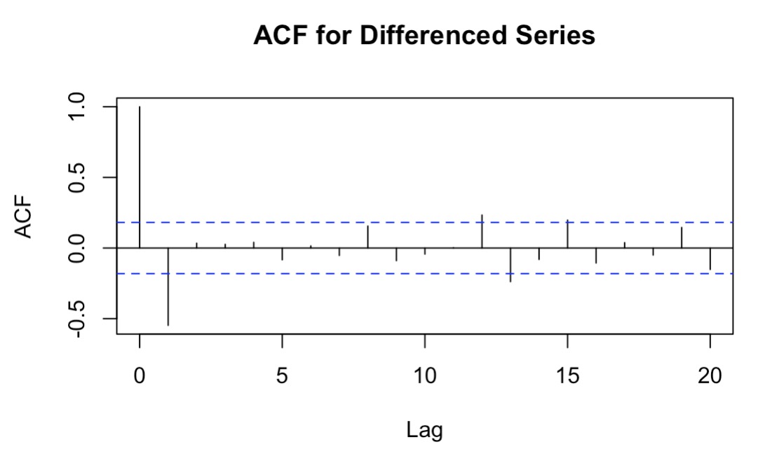
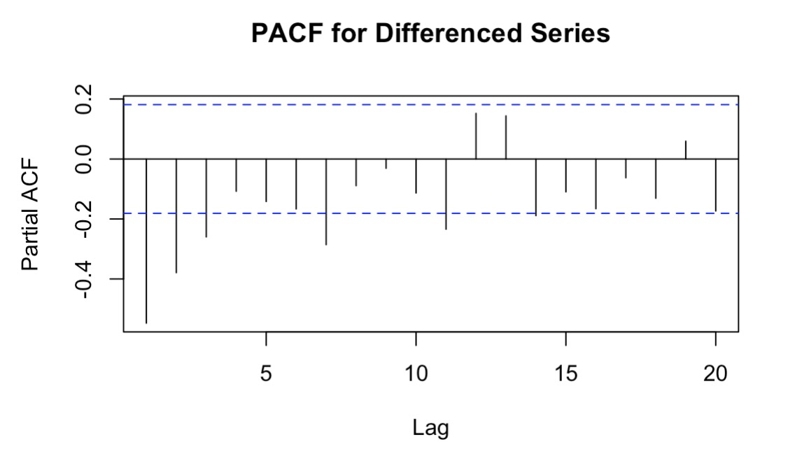
Before making predictions, this paper needs to first determine the various parameters of the model. The first step is to determine the p and q values in the model. Since ARIMA model requires time series to be stationary, ADF test was conducted to assess the stationarity of data [7]. Time series stationarity can be effectively assessed using ACF and PACF plots. A slow decay in the ACF plot indicates that the time series is non-stationary [8]. Based on the ACF and PACF methods, this paper can preliminarily determine the approximate range of p and q.

From the Figures 2 and 3, preliminary estimates for the parameters p and q can be deduced, with both approximately equal to 1. This inference is drawn from the observation that the coefficients at the first lag are statistically significant, as they lie outside the confidence intervals. In contrast, the coefficients at higher lags are all contained within their respective confidence intervals, indicating their lack of statistical significance. Typically, the ACF and PACF of a model manifest in one of two conditions: they either trail off or are truncated. When the ACF or PACF drops to zero following a specific lag—denoted as p or q—it is characterized as truncated. Conversely, when these functions exhibit a geometric decline toward zero as the lag order k ascends, this is referred to as a trailing pattern [9].

According to the AIC and BIC methods, in this paper, the values of p and q are both set between 0 and 5, and then AIC and BIC are selected to achieve the minimum combination simultaneously. Therefore, it was finally determined to use the ARIMA (0,2,1) model. After constructing the model, this paper needs to test the residual terms of the model to verify whether the residual terms are white noise. If the residual terms are white noise, it indicates that the constructed model is reasonable; otherwise, further adjustments are required. From Table 1, it can be clearly seen that all p-values are greater than 0.05, indicating that the residual terms are white noise and the model can be used for final prediction.

Finally, to verify whether the order of the model is reasonable, this paper will conduct an overfitting test on the model to avoid bias in the final results due to an excessively high order. As shown in Table 2, the result of the overfitting test is 0.00, which is less than 0.05. Therefore, the model does not have an overfitting problem, and the final prediction can be made.

4.4. Model forecast

Subsequently, the model is employed for forecasting purposes. In this study, predictions for the opening stock prices of Pop Mart for the subsequent 7 days are derived (as shown in Figure 4). In Figure 4, the light grey region delineates the 80% confidence interval, while the blue-grey area represents the 95% confidence interval.

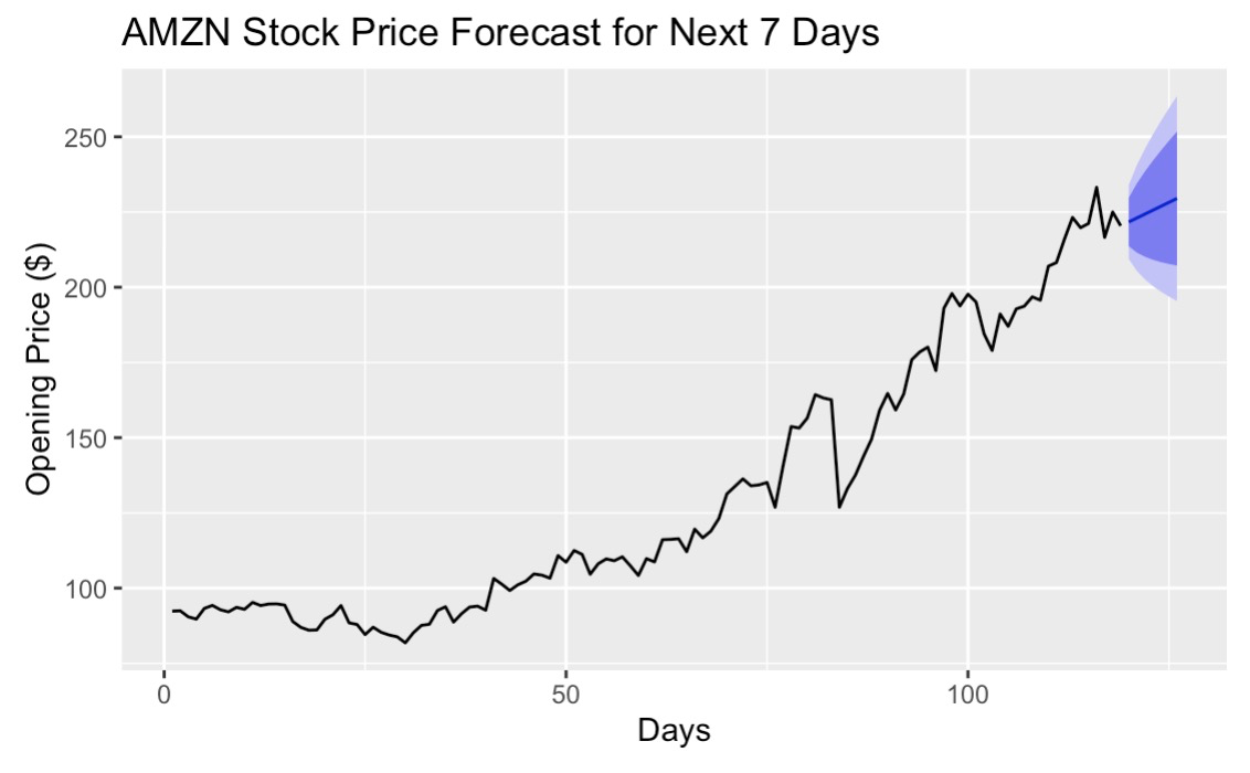
Then Table 3 lists the specific prediction data and results under 80% and 95% confidence intervals.

Subsequently, this article collects the actual values of the company's stocks on the corresponding dates and calculates the error between the predicted values and the actual values, as shown in Table 4. It can be seen that the MAPE value is 8.29%, which is less than 10%. Therefore, it indicates that the predictions are relatively accurate [10]. At the same time, according to the model's predictions, the stock price of Bubble Code Company will show an upward trend in the future, and the actual results also show an upward trend. This shows that the results obtained by the model have high reference value.

5. Conclusion

The stock market is crucial to many aspects of economic activity. It serves as an efficient mechanism for the allocation of capital to sectors and enterprises that demonstrate superior performance and growth prospects, thereby facilitating optimal resource distribution. Furthermore, the equity market aids businesses in expanding their operational scale, which in turn generates additional employment opportunities. This expansion can lead to the development of vertical and horizontal industry linkages, fostering the formation of industrial clusters and contributing to the overall economic expansion. The stock market also functions as a barometer of macroeconomic health, with stock price movements providing insights into broader economic trends. For both corporate entities and investors, the stock market is of significant relevance, underscoring the importance of accurate stock market forecasting. This study employs a time series analysis to construct an ARIMA (p, d, q) model for predictive purposes. Focusing on the stock performance of Pop Mart from December 2024 to May 2025, an ARIMA (0,2,1) model was developed to forecast the opening prices for the subsequent five days. The model achieved a MAPE of 8.29%, which is considerably below the 10% threshold, indicating a high level of forecasting accuracy.

This research represents a foundational exploration, yet it acknowledges the complexity and volatility inherent in the securities market, suggesting that future studies should address additional considerations. Firstly, the study's scope is limited to the opening prices, neglecting other pertinent variables such as closing prices, high and low prices, and trading volume. Moreover, external factors that can substantially influence stock prices, especially in relation to industry trends, were not taken into account. The omission of these elements may hinder the precise capture of price dynamics driven by trading volume fluctuations. To enhance the precision of predictions, it is recommended to integrate this model with other methodologies. For example, Long Short-Term Memory (LSTM) networks. The LSTM's robust capacity for non-linear modeling, when combined with the ARIMA model's strength in linear trend fitting, can provide a more comprehensive depiction of stock price patterns, thereby improving the accuracy of forecasts.

References

[1]. Al-Musaylh, M.S., Deo, R.C., Adamowski, J.F. and Li, Y. (2018) Short-Term Electricity Demand Forecasting with MARS, SVR and ARIMA Models using Aggregated Demand Data in Queensland, Australia. Advanced Engineering Informatics, 35, 1-16.
[2]. Liapis, C.M., Karanikola, A. and Kotsiantis, S. (2021) A Multi-Method Survey on the use of Sentiment Analysis in Multivariate Financial Time Series Forecasting. Entropy (Basel, Switzerland), 23, 1603.
[3]. Wang, X., Kang, Y., Hyndman, R.J. and Li, F. (2023) Distributed ARIMA Models for Ultra-long Time Series. International Journal of Forecasting, 39, 1163-1184.
[4]. Pokou, F., Sadefo Kamdem, J. and Benhmad, F. (2024) Hybridization of ARIMA with Learning Models for Forecasting of Stock Market Time Series. Computational Economics, 63, 1349-1399.
[5]. Funde, Y. and Damani, A. (2023) Comparison of ARIMA and Exponential Smoothing Models in Prediction of Stock Prices. Journal of Prediction Markets, 17, 21–38.
[6]. Khan, K. (2022) Stock Price Forecasting of Maruti Suzuki using ARIMA Model. Parikalpana: KIIT Journal of Management, 18, 90–98.
[7]. Erker, E. (2024) Forecasting Medical inflation in the European Union using the ARIMA model. Public Sector Economics, 48, 39–56.
[8]. Singh, S., Parmar, K. S. and Kumar, J. (2021) Soft Computing Model Coupled with Statistical Models to Estimate Future of Stock Market. Neural Computing & Applications, 33, 7629–7647.
[9]. Ning, L., Pei, L., Li, F. and Xie, L. (2021) Forecast of China’s Carbon Emissions Based on ARIMA Method. Discrete Dynamics in Nature and Society, 2021, 1–12.
[10]. Dun, V. (2023) Analysis and Forecasting the Price of the S&P 500 Index Using the Arima Model. Financial Markets, Institutions and Risks, 7, 113–134.
Cite this article
Sha,Y. (2025). Analyze the Future Stock Trend of Pop Mart Based on the Time Series Model. Advances in Economics, Management and Political Sciences,207,1-7.
Data availability
The datasets used and/or analyzed during the current study will be available from the authors upon reasonable request.
Disclaimer/Publisher's Note
The statements, opinions and data contained in all publications are solely those of the individual author(s) and contributor(s) and not of EWA Publishing and/or the editor(s). EWA Publishing and/or the editor(s) disclaim responsibility for any injury to people or property resulting from any ideas, methods, instructions or products referred to in the content.
About volume
Volume title: Proceedings of ICEMGD 2025 Symposium: Innovating in Management and Economic Development
© 2024 by the author(s). Licensee EWA Publishing, Oxford, UK. This article is an open access article distributed under the terms and
conditions of the Creative Commons Attribution (CC BY) license. Authors who
publish this series agree to the following terms:
1. Authors retain copyright and grant the series right of first publication with the work simultaneously licensed under a Creative Commons
Attribution License that allows others to share the work with an acknowledgment of the work's authorship and initial publication in this
series.
2. Authors are able to enter into separate, additional contractual arrangements for the non-exclusive distribution of the series's published
version of the work (e.g., post it to an institutional repository or publish it in a book), with an acknowledgment of its initial
publication in this series.
3. Authors are permitted and encouraged to post their work online (e.g., in institutional repositories or on their website) prior to and
during the submission process, as it can lead to productive exchanges, as well as earlier and greater citation of published work (See
Open access policy for details).