1. Introduction

In their seminal work, Black and Scholes showed that under certain idealized conditions (constant volatility, frictionless trading, continuous time), an option’s payoff can be perfectly replicated by continuously adjusting a portfolio of the underlying asset and risk-free asset [1]. This continuous delta hedging strategy leads to a riskless portfolio and yields the celebrated Black–Scholes option pricing formula. Merton extended this theory, and together they demonstrated that, if the model assumptions hold, the cost of hedging an option (i.e., the initial option premium) equals the option’s arbitrage-free price [2]. The necessary conditions for perfect hedging include a single source of uncertainty (the underlying’s price following a geometric Brownian motion with constant volatility) and no market frictions. Under these conditions, the market is complete and admits a unique risk-neutral pricing measure.

However, financial markets in reality violate several Black–Scholes assumptions. Two important deviations are stochastic volatility and jump discontinuities in asset prices. Empirical evidence shows that asset return distributions exhibit excess kurtosis (fat tails) relative to the lognormal, and volatility is time-varying and stochastic. To address these phenomena, more complex models have been developed. Notably, jump–diffusion models introduce sudden price jumps [2], and continuous-time stochastic volatility models introduce additional randomness in volatility [3]. These richer models can better fit market option price patterns such as implied volatility skews and smiles. However, they also make the market incomplete – there are now multiple sources of uncertainty (e.g. a volatility factor or jump shocks) but only one primary asset available for hedging. In an incomplete market, a contingent claim cannot be perfectly hedged using only the underlying asset. As a result, there is no unique arbitrage-free price; instead, a continuum of fair prices exists, and hedging strategies can only minimize risk rather than eliminate it.

Practitioners have responded to incompleteness in various ways. One approach is to augment the hedging portfolio with additional instruments—for example, using traded options to hedge jump risk or volatility risk in addition to the underlying stock. It has been shown that holding a short-term option in the hedge portfolio can significantly mitigate jump-induced losses [4]. Such multi-instrument hedging can, in theory, restore completeness if a sufficient set of contingent claims is available (e.g. using a vanilla option to hedge Vega exposure in an SV model). Another approach is to accept that some risk is unhedgeable and to seek an optimal hedge that balances risk and cost. Strategies like mean-variance hedging and quadratic risk minimization explicitly choose the hedge ratio that minimizes the variance of the hedging error, rather than using the Black–Scholes delta. These optimal hedge ratios generally differ from Black–Scholes delta and do not fully eliminate risk, but they minimize it under a given criterion.

Even setting aside model incompleteness, discrete-time hedging (in contrast to continuous rebalancing) introduces additional imperfection. In practice, hedging adjustments occur at finite intervals (e.g., daily) rather than continuously. Studies have examined the discretization error associated with infrequent rebalancing [5-7]. They found that discretely rebalanced hedges lead to a distribution of final hedging costs or errors, rather than a single deterministic cost equal to the option’s price. In a Black–Scholes world (no jumps, constant vol), the average outcome of a high-frequency discrete hedge still equals the Black–Scholes price, but there is appreciable variance around this mean cost. This variance grows as the rebalancing interval lengthens (i.e. hedging less frequently), and it represents the residual risk of a discrete hedge.

Another crucial consideration is transaction costs. Continuous hedging is infeasible and would imply infinite trading costs under frictions. Even a very small proportional cost per trade can drastically alter hedging strategy and option pricing [6]. Frequent trading becomes expensive, prompting the question of an optimal rebalancing frequency that balances risk reduction against cost. Modified option-pricing equations under transaction costs have been derived, effectively widening the no-arbitrage bounds to account for the cost–risk trade-off [8, 9]. In general, with transaction costs present, hedging strategies that are too aggressive (trading on every tiny price move) may over-hedge, spending more on transactions than the incremental risk reduction is worth. On the other hand, hedging too infrequently leaves substantial risk. Thus, there is an intuitive trade-off between cost and risk in choosing a hedging policy.

In an incomplete market setting with jumps or SV (or both) and with transaction costs, the problem becomes finding a strategy that optimally compromises between risk and cost. Recent research has addressed this problem from various angles. For instance, stochastic control and model predictive control approaches have been applied to hedging with cost penalization, yielding a Pareto-optimal frontier of strategies [10]. More directly, “restricted but optimal” delta hedging under scenarios including jumps, stochastic volatility, and transaction costs has been investigated [7]. In his analysis, the hedge is only adjusted at discrete intervals and can incorporate realistic costs; the optimal strategy is one that minimizes a combination of hedging error variance and cost. Such studies confirm that incorporating jumps and volatility risk leads to a non-zero minimum attainable risk – even the best strategy cannot eliminate risk completely, because some sources of uncertainty remain unhedged. They also underscore that the relationship between how often one hedges and the resulting cost and risk is nonlinear: beyond a certain point, more frequent hedging yields only marginal risk reduction but incurs significantly higher costs.

This paper contributes to the literature by explicitly quantifying the cost–risk frontier for discrete delta hedging in a model that includes both stochastic volatility and jumps. It uses Monte Carlo simulation to evaluate hedging performance across a range of rebalancing frequencies, from very frequent (approaching continuous) to very sparse. For each frequency, it computes the expected transaction cost incurred and the residual risk (measured by the standard deviation of final hedging P&L). Plotting these as a trade-off curve yields the frontier: strategies on the frontier are Pareto-optimal in the sense that you cannot reduce risk without increasing cost, or reduce cost without increasing risk. This provides a concrete illustration of the principle that “there is no free lunch” in incomplete markets – any reduction in risk must be paid for, either via higher cost or via accepting some other form of risk.

The remainder of the paper is organized as follows. In Section 2, it describes the market model (stochastic volatility with jumps) and the discrete delta hedging strategy, including how we incorporate transaction costs. Section 3 details the Monte Carlo simulation approach and parameter choices. In Section 4, it presents the results, including the cost–risk frontier chart obtained and discussion of its shape. Section 5 concludes with insights on practical hedging policy implications and potential extensions of this work.

2. Model and methodology

Underlying Asset Dynamics: It assumes the underlying asset St follows a stochastic volatility jump-diffusion process. Specifically, we adopt a variant of the Bates model [11]. Under the risk-neutral measure, the dynamics are:

• Stochastic volatility: $$ \mathrm{d}{\mathrm{V}}_{\mathrm{t}}=\mathrm{\kappa }\left(\mathrm{\theta }-{\mathrm{V}}_{\mathrm{t}}\right),\mathrm{d}\mathrm{t}+\mathrm{\eta }\sqrt{{\mathrm{V}}_{\mathrm{t}}},\mathrm{d}{\mathrm{W}}_{\mathrm{t}}^{\mathrm{V}}$$, where  $$ {\mathrm{V}}_{\mathrm{t}}$$  is the instantaneous variance,  $$ \mathrm{\kappa }$$  is the mean-reversion rate, theta the long-run mean variance,  $$ \mathrm{\theta }$$vol-of-vol, and  $$ {\mathrm{W}}_{\mathrm{t}}^{\mathrm{V}}$$ a Wiener process. This is the Heston SV model for volatility. We assume the Feller condition for  $$ {\mathrm{V}}_{\mathrm{t}}$$  to stay positive. The correlation between the volatility shock  $$ \mathrm{d}{\mathrm{W}}_{\mathrm{t}}^{\mathrm{V}}$$  and the asset price shock  $$ \mathrm{d}{\mathrm{W}}_{\mathrm{t}}^{\mathrm{S}}$$  is  $$ \mathrm{\rho }$$  (which may be zero or negative as commonly estimated in equity markets).

• Jump component: In addition to the diffusive price shock, we include jumps via a Poisson process$$ {\mathrm{N}}_{\mathrm{t}}$$with intensity$$ \mathrm{\lambda }$$(jumps per year). When a jump occurs, the asset price experiences a multiplicative jump $$ \mathrm{J}={\mathrm{e}}^{\mathrm{Y}}$$, where  $$ \mathrm{Y}$$  is a random jump size (we assume $$ \mathrm{Y}\sim \mathrm{N}\left({\mathrm{\mu }}_{\mathrm{J}},{\mathrm{\sigma }}_{\mathrm{J}}^2\right)$$ , i.e., log-normal jumps). Thus,  $$ {\mathrm{S}}_{\mathrm{t}}$$  satisfies:

$$ \text{d}{S}_t=S_t\left(r\hspace{0.17em}\text{d}t+\sqrt{V_t}\hspace{0.17em}\text{d}{W}_t^S+\left(J-1\right)\hspace{0.17em}\text{d}{N}_t\right)$$(1)

where  $$ \mathrm{r}$$  is the risk-free rate. We choose  $$ {\mathrm{\mu }}_{\mathrm{J}}$$ such that  $$ \mathrm{E}\left[\mathrm{J}-1\right]=0$$  under the risk-neutral measure (so on average jumps do not drift the price), and  $$ {\mathrm{\sigma }}_{\mathrm{J}}$$  controls jump volatility. Jumps arriving with intensity  $$ \mathrm{\lambda }$$  make the price process exhibit sudden discontinuities, contributing to heavier tails and skewness in returns.

This model incorporates two independent risk factors: the Brownian diffusive risk (with stochastic variance) and the jump risk. With only the underlying stock available to trade (and perhaps a money market account), the market is incomplete. There is no trading strategy in  $$ {\mathrm{S}}_{\mathrm{t}}$$  alone that can hedge a derivative perfectly, even with continuous trading. Intuitively, continuous delta-hedging can neutralize the instantaneous diffusion risk (the  $$ \mathrm{d}{\mathrm{W}}_{\mathrm{t}}^{\mathrm{S}}$$  term) but cannot foresee jumps — any jump will cause a discontinuous change in S that leads to a hedging error. Likewise, unpredictable changes in volatility  $$ {\mathrm{V}}_{\mathrm{t}}$$  will alter the option’s value in ways that cannot be offset by just trading  $$ {\mathrm{S}}_{\mathrm{t}}$$  This inherent limitation means a delta-hedged portfolio will still exhibit random P&L fluctuations.

Option and Hedging Setup: For concreteness, we consider hedging a short position in a European call option on  $$ S$$  (strike  $$ K$$ , maturity  $$ T$$). The initial option premium (theoretical fair price) is denoted C₀. In our risk-neutral simulation, $$ {\mathrm{C}}_0$$is computed as the expected discounted payoff $$ {\mathrm{e}}^{-\mathrm{r}\mathrm{T}}\mathrm{E}\left[{\left({\mathrm{S}}_{\mathrm{T}}-\mathrm{K}\right)}^{+}\right]$$. At time 0, the hedger sells the call for$$ {\mathrm{C}}_0$$and begins a delta-hedging strategy. The strategy is discrete delta hedging, meaning we choose a sequence of rebalancing times$$ 0={\mathrm{t}}_0<{\mathrm{t}}_1<\dots <{\mathrm{t}}_{\mathrm{N}}=\mathrm{T}$$  at which the hedge ratio is updated. Between these times, the holdings are fixed. At each hedge time  $$ {\mathrm{t}}_{\mathrm{i}}$$, we set the position in the underlying stock to $$ \mathrm{\Delta }\left({\mathrm{t}}_{\mathrm{i}}\right)$$, where $$ \mathrm{\Delta }\left(\mathrm{t}\right)$$is an estimate of the option’s delta (sensitivity to $$ \mathrm{S}$$). In a complete-market setting, the ideal delta would be the partial derivative $$ \partial \mathrm{C}/\partial \mathrm{S}$$  given the model. In our setting, one could use the theoretical delta from a model (if available in closed form via Heston's formula or simulation). For simplicity, we use an approximate delta given by the Black–Scholes formula, but updated at each time with the current observed volatility level. Specifically, we compute:

$$ \mathrm{\Delta }\left({\mathrm{t}}_{\mathrm{i}}\right)=\mathrm{N}\left({\mathrm{d}}_1\left({\mathrm{S}}_{{\mathrm{t}}_{\mathrm{i}}},{\mathrm{V}}_{{\mathrm{t}}_{\mathrm{i}}},\mathrm{T}-{\mathrm{t}}_{\mathrm{i}}\right)\right)$$(2)

where N(·) is the standard normal CDF (the Black–Scholes delta for a call), and $$ {\mathrm{d}}_1\left(\mathrm{S},\mathrm{\sigma },\mathrm{\tau }\right)=\frac{\mathrm{l}\mathrm{n}\left(\mathrm{S}/\mathrm{K}\right)+\frac{1}{2}{\mathrm{\sigma }}^2\mathrm{\tau }}{\mathrm{\sigma }\sqrt{\mathrm{\tau }}}$$,

with$$ \mathrm{\sigma }=\sqrt{{\mathrm{V}}_{{\mathrm{t}}_{\mathrm{i}}}}$$  interpreted as the current volatility and $$ \mathrm{\tau }=\mathrm{T}-{\mathrm{t}}_{\mathrm{i}}$$  the remaining time. This approach effectively treats the local volatility as $$ {\mathrm{\sigma }}_{\text{loc}}=\sqrt{{\mathrm{V}}_{{\mathrm{t}}_{\mathrm{i}}}}$$  and computes a Black–Scholes delta with that volatility. While not exact (since the true optimal delta in stochastic volatility differs), this mimics common practice where traders update greeks based on current implied or local volatilities. It also ensures $$ \mathrm{\Delta }\left(\mathrm{t}\right)$$evolves in a plausible manner between 0 and 1 depending on moneyness and time. At maturity, we do not rebalance (the option payoff is realized).

Trading Costs: Each time the hedge is adjusted, the change in the stock position incurs a transaction cost. We assume a simple proportional cost model: whenever $$ \mathrm{\Delta }$$  is changed, the trader pays a cost equal to a fraction  $$ \mathrm{\alpha }$$  of the dollar value of stock traded. For example, if at time$$ {\mathrm{t}}_{\mathrm{i}-1}$$  the position was $$ {\mathrm{\Delta }}_{\mathrm{i}-1}$$  and at  $$ {\mathrm{t}}_{\mathrm{i}}$$  the new target is  $$ {\mathrm{\Delta }}_{\mathrm{i}}$$, and the stock price at $$ {\mathrm{t}}_{\mathrm{i}}$$  is$$ {\mathrm{S}}_{{\mathrm{t}}_{\mathrm{i}}}$$, then:

$transactioncost=\alpha ,\mathrm{\mid },\mathrm{\Delta }\mathrm{\_}i-\mathrm{\Delta }\mathrm{\_}\{i-1\},\mathrm{\mid },S_{t_i}\mathrm{.}$(3)

This can represent a bid–ask spread or commission. In our simulations, we take a modest  $$ \alpha $$  (e.g., 0.1% per trade), but accumulated over many trades this can meaningfully erode profits. The presence of transaction costs discourages extremely frequent rebalancing — the incremental risk reduction from an extra rebalance must be weighed against the certain cost incurred.

Hedging P&L: The performance of the hedging strategy is evaluated by the profit-and-loss (P&L) at option expiration. We track the replicating portfolio consisting of$$ \mathrm{\Delta }\left(\mathrm{t}\right)$$shares of stock and a cash account (financing the stock purchases or generated from stock sales). Starting with initial cash$$ {\mathrm{C}}_0$$(from selling the option) and$$ \mathrm{\Delta }\left(0\right)$$shares, the portfolio is rebalanced at each$$ {\mathrm{t}}_{\mathrm{i}}$$. Between hedges, the stock holding $$ \mathrm{\Delta }\left({\mathrm{t}}_{\mathrm{i}-1}\right)$$grows in value as  $$ S$$  moves, and the cash earns interest at rate$$ r$$(here we set  $$ r$$  low or zero for simplicity). At  $$ {\mathrm{t}}_{\mathrm{i}}$$ , we adjust the stock holding by  $$ {\mathrm{\Delta }}_{\mathrm{i}}-{\mathrm{\Delta }}_{\mathrm{i}-1}$$ , and the cash account changes by the negative of the stock trade plus the transaction cost. At  $$ T$$ , the short call position is settled by paying the payoff  $$ {\left({\mathrm{S}}_{\mathrm{T}}-\mathrm{K}\right)}^{+}$$to the option holder. The hedging error (final P&L) is:

$$ \mathrm{\Pi }=\left(\text{value of stock}+\text{cash}\right)-\left(\text{option payoff liability}\right)$$(4)

If  $$ \mathrm{\Pi }=\mathrm{ }0$$, the hedge perfectly replicated the payoff; $$ \mathrm{\Pi }>\mathrm{ }0$$  indicates a profit for the hedger (the strategy over-hedged), and $$ \mathrm{\Pi }<\mathrm{ }0$$  a loss (under-hedged). In an ideal frictionless complete-market world, we would have $$ \mathrm{\Pi }=\mathrm{ }0$$  deterministically for the correct strategy. In our incomplete, discrete, costly setting,  $$ \mathrm{\Pi }$$is a random variable. We focus on its mean and standard deviation as key metrics. The mean $$ \mathrm{E}\left[\mathrm{\Pi }\right]$$  represents any systematic bias (which in our case comes mostly from transaction costs — we expect $$ \mathrm{E}\left[\mathrm{\Pi }\right]<0$$, i.e., an average loss equal to the total cost paid by the hedger, since the initial option price was fair). The standard deviation  $$ {\mathrm{\sigma }}_{\mathrm{\Pi }}$$  measures the risk — the volatility of the hedging outcome. A well-chosen hedge will have a small  $$ {\mathrm{\sigma }}_{\mathrm{\Pi }}$$ , indicating outcomes tightly clustered around the mean (ideally around zero or a small negative cost). We will use  $$ {\mathrm{\sigma }}_{\mathrm{\Pi }}$$  as our metric of residual risk, and the average transaction cost$$ \mathrm{E}\left[\text{cost}\right]=-\mathrm{E}\left[\mathrm{\Pi }\right]$$  as our cost measure (since any shortfall in P&L for the hedger is essentially the cost expended, assuming zero drift under risk-neutral pricing).

3. Simulation and implementation

To investigate the cost–risk trade-off, we perform a Monte Carlo simulation for various hedging frequencies, and the corresponding results are shown in Table 1. It fixes a set of model parameters for illustration: an initial stock price$$ {\mathrm{S}}_0=100$$, option strike  $$ \mathrm{K}\mathrm{ }=\mathrm{ }100$$(at-the-money), maturity $$ \mathrm{T}\mathrm{ }=\mathrm{ }1$$year. Volatility starts at  $$ {\mathrm{V}}_0=0.04$$  (so 20% initial vol). It chooses Heston parameters $$ \mathrm{\kappa }=\mathrm{ }1.0$$, $$ \mathrm{\theta }=\mathrm{ }0.04$$, $$ \mathrm{\eta }=\mathrm{ }0.2$$, and correlation$$ \mathrm{\rho }=\mathrm{ }0$$  (uncorrelated for simplicity). Jump parameters are$$ \mathrm{\lambda }=\mathrm{ }1.0$$(on average one jump per year),  $$ {\mathrm{\sigma }}_{\mathrm{J}}=0.25$$(so about 25% jump size volatility), and  $$ {\mathrm{\mu }}_{\mathrm{J}}=-0.5{\mathrm{\sigma }}_{\mathrm{J}}^2$$ (approximately −0.03125) to ensure mean jump size is 1 (no drift). The transaction cost rate is set to  $$ \mathrm{\alpha }=\mathrm{ }0.001$$ (0.1% of traded value each hedge).

For each strategy, it simulates a large number of price paths (on the order of 50,000 or more) to accurately estimate the distribution of P&L. Each path is generated by discretizing the SDEs for  $$ S_t$$  and  $$ V_t$$  on a daily time grid ( $$ \mathrm{\Delta }\mathrm{t}=\frac{1}{252}$$ ). We use an Euler discretization for the volatility process and incorporate jumps by a simple Poisson sampling each day (if a jump occurs during a day, we multiply  $$ S$$  by the jump factor  $$ J$$ ). The delta hedge is applied by sampling the state at the designated hedge times and rebalancing accordingly.

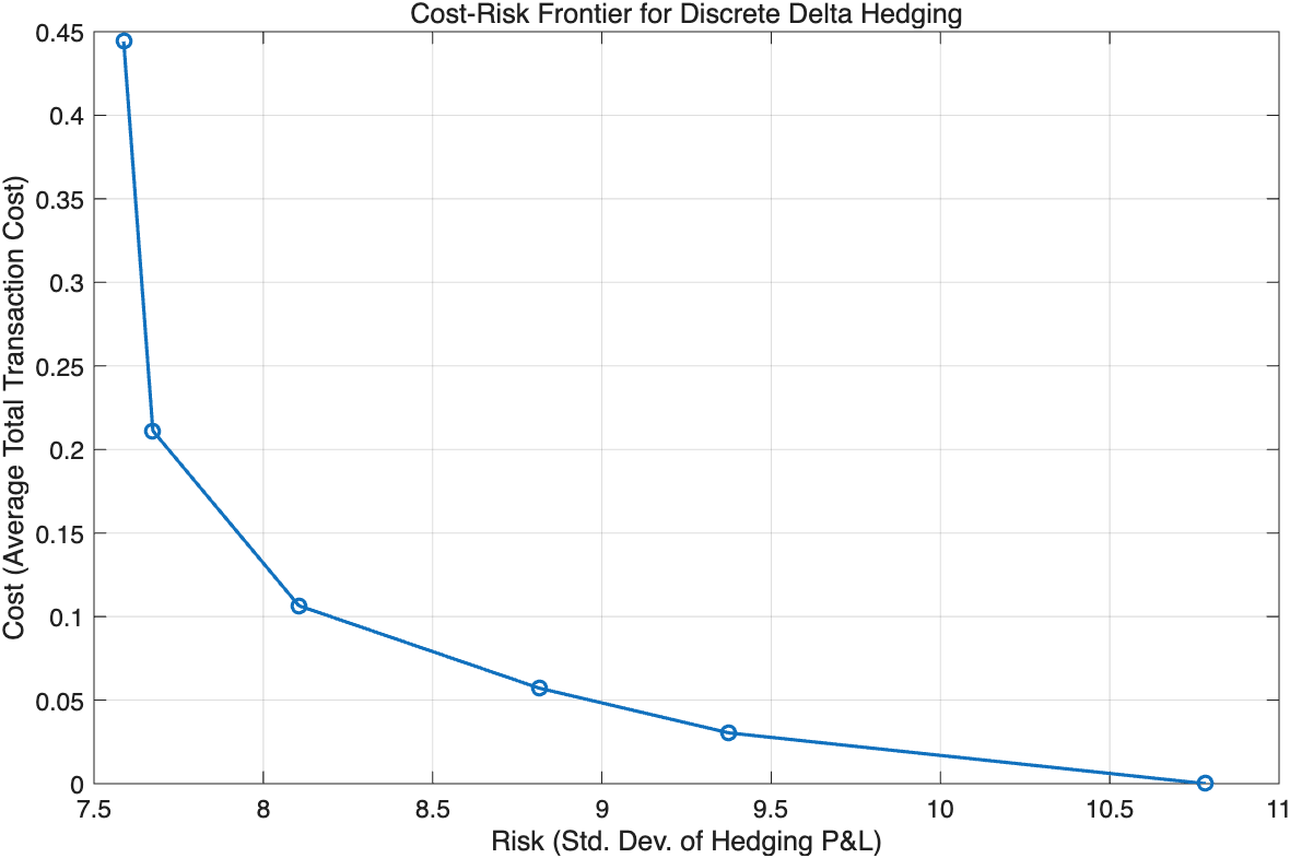
The entire simulation and analysis were implemented in MATLAB. Figure 1 reports the cost–risk frontier generated by our Monte Carlo engine for the parameter set described in the Model and Methodology section. The algorithm simulates Bates dynamics (Heston stochastic volatility with Merton-type jumps) on a daily grid, applies discrete delta hedging at the stated rebalancing intervals with proportional transaction costs, and records terminal hedging P&L across simulated paths. For reproducibility, it initializes the MATLAB random number generator to a fixed state (seed 123456, twister stream). The fully annotated script and run instructions are provided in the Supplementary Material (and mirrored at the public repository listed in “Data and Code Availability”).

The simulation evolves price and variance path-by-path and computes the P&L for each hedging frequency; we use  $$ {10}^5$$  paths for the final estimates to control Monte Carlo error. Mean transaction cost and the standard deviation of the hedging P&L are computed for each frequency, and the resulting pairs are plotted in Figure 1 to form the empirical cost–risk frontier. To improve efficiency and comparability across frequencies, we employ vectorization and common random numbers; Figure 1 was exported from MATLAB in vector format for publication quality.

4. Results and discussion

As Figure 1 shows, Monte Carlo estimated cost–risk frontier for discrete delta hedging under stochastic volatility and jumps. The x-axis is the risk (standard deviation of hedging P&L) and the y-axis is the cost (average total transaction costs incurred). Each labeled point corresponds to a different hedging frequency (e.g. daily, weekly, monthly, etc.). The curve illustrates the trade-off: achieving lower risk requires higher cost. Notably, the frontier is nonlinear, showing diminishing risk reduction returns for increasing cost.

The cost–risk frontier obtained from the simulation is shown in Figure 1. Each point on the plot represents one hedging strategy parameterized by rebalancing frequency. The rightmost point (highest risk, lowest cost) corresponds to a buy-and-hold strategy with essentially no rebalancing (in our case, an initial delta hedge set at  $$ t=0$$  and never adjusted, which is analogous to annual hedging for a 1-year option). The leftmost point (lowest risk, highest cost) corresponds to daily hedging. As expected, more frequent hedging moves the outcome towards lower risk: the standard deviation of P&L for daily hedging is substantially smaller than for monthly or quarterly hedging. Meanwhile, the cumulative transaction costs for daily hedging are much higher than for infrequent hedging.

Here the frontier delivers four big takeaways. First, even very frequent rebalancing cannot eliminate risk: jumps (gap risk) and stochastic volatility (unspanned vega risk) leave an irreducible hedging error when you hedge only with the underlying. Second, increasing hedge frequency exhibits strong diminishing returns—moving from very infrequent to moderate rebalancing slashes risk, but beyond that the curve flattens and extra trades mostly buy small variance reductions. Third, transaction costs reshape the optimum: because every adjustment burns cash and adds cost variability, extremely frequent hedging can raise total risk after costs; the efficient choice is an interior cadence on the flat part of the frontier where the marginal risk reduction roughly equals the marginal cost. Fourth, the mean P&L is negative across strategies, effectively matching average transaction costs, so delta hedging behaves like paying an insurance premium to compress tails rather than a profit center.

Managerially, the slope of the frontier at a candidate cadence is the “price of risk reduction.” Choose the frequency where that price aligns with risk appetite or capital constraints. Parameter shifts move the whole curve: more frequent/larger jumps or higher vol-of-vol push it right (more residual risk), while higher trading frictions push it up (greater cost). Thus, a jumpier asset or wider spreads warrant less aggressive rebalancing; quieter markets with tight spreads can justify more. If deeper risk cuts are required, adding a second instrument (e.g., a short-dated option for vega/jump exposure) doesn’t change the trade-off logic but can shift the entire frontier inward, achieving lower risk for the same cost.

Overall, the cost–risk frontier quantifies the intuitive idea that you can buy reduced risk by paying higher transaction cost. Each point on the frontier could be seen as an efficient hedging strategy for a particular risk tolerance: a risk-averse hedger might choose a high-frequency, high-cost strategy to minimize variance, whereas a cost-sensitive (or less risk-averse) hedger might accept more risk in exchange for lower costs.

It is important to note that the exact shape and numbers on the frontier will depend on model parameters (volatility of volatility, jump intensity, etc.) and on the option’s characteristics (maturity, strike). For instance, a higher jump intensity  $$ \mathrm{\lambda }$$  or larger jump size  $$ {\mathrm{\sigma }}_{\mathrm{J}}$$  would increase the residual risk for all strategies (shifting the frontier rightwards – more risk) because jumps are harder to hedge. A higher transaction cost rate  $$ \mathrm{\alpha }$$  would make the high-frequency strategies even more costly (shifting the frontier upwards – more cost). The frontier we present is thus illustrative, but the methodology can be applied to specific situations to determine an appropriate hedging frequency or to estimate the efficient frontier for that scenario.

Our findings are consistent with previous analytical results in the literature. As Merton (1976) pointed out, in a jump-diffusion setting a delta-hedged portfolio will still experience jumps in value leading to losses. Our simulation shows those losses manifest as a baseline level of risk that cannot be diversified away by faster trading. Similarly, the transaction cost effects we observe align with Leland’s theory that effective volatility is increased by transaction costs – in other words, the presence of costs makes it as if the option is riskier, because one cannot chase the deltas as closely. What we see in the frontier’s flattening is essentially that phenomenon: beyond a point, increasing hedge frequency yields minimal risk reduction because effectively the strategy is “running in place” – incurring costs to shave off ever smaller risk components.

One interesting aspect worth discussing is that in our simulation we used a simple Black–Scholes delta estimate. One could ask: would using a more optimal delta (for example, the mean-variance optimal hedge ratio given the model) improve the trade-off? Potentially yes – an optimal strategy could achieve a lower variance for the same cost. In that case, our frontier would shift towards the origin (improvement). However, the general shape would remain – there would still be a convex, diminishing-return curve. Our focus here was on delta hedging as it is a common baseline. Future work could incorporate optimal hedging rules or non-linear instruments to see how the frontier shifts (for example, adding a second instrument like a short-term put might allow further risk reduction, effectively pushing the frontier downward at the low-risk end by completing more of the market).

We also note that the distribution of hedging P&L (not just its variance) is of interest. In our simulation, the unhedged position (short call without any hedge) would have a very dispersed P&L distribution, effectively the negative of the call’s payoff distribution. Hedging narrows this distribution. We observed that with daily hedging, the P&L distribution becomes more concentrated around a small loss (the cost), whereas with monthly hedging the distribution is wider. Hedging particularly trims the extreme tail outcomes – for example, scenarios where the stock price skyrockets at expiration (which would be a huge loss for an unhedged short call) are substantially mitigated by delta hedging, since the hedger would have acquired a lot of stock in those scenarios. However, jump risk implies that a sudden large move just before a hedge adjustment can still produce a significant loss. This highlights that while delta hedging addresses continuous price risk effectively, it is less effective for gap risk. In practice, risk managers often complement delta hedging with other tools (like stop-loss rules or options positions) to handle jump risk.

5. Conclusion

Here we examined discrete-time delta hedging in an equity market with stochastic volatility and jumps, using Monte Carlo simulation to map the trade-off between hedging cost and residual risk. Unlike the idealized Black–Scholes setting—where continuous rebalancing with constant volatility yields exact replication—the presence of volatility randomness and discontinuous price jumps makes the market intrinsically incomplete. Even with very frequent rebalancing, a nontrivial, irreducible variance of the hedging error persists because trading the underlying alone cannot span volatility and jump risks. Discreteness compounds this limitation: in a Black–Scholes world, discrete hedging produces a distribution of replication outcomes with zero mean and nonzero variance; in our richer setting, proportional transaction costs push the mean outcome negative while leaving a wider dispersion of P&L. As trading frequency increases, variance typically falls, but at a diminishing rate, while costs climb quickly; beyond moderate frequencies, additional rebalancing primarily purchases marginal risk reduction at disproportionate expense. The resulting cost–risk frontier makes this trade-off explicit, tracing the Pareto set of efficient strategies from low-cost/high-risk to high-cost/low-risk. This frontier offers a practical decision tool: risk managers can select a rebalancing cadence consistent with their risk appetite and cost budget, or assess whether a targeted variance reduction justifies the incremental transaction cost. The framework is readily extensible. The same simulation engine can be adapted to different maturities and strikes, to alternative instruments (e.g., American-style contracts, bearing in mind early-exercise complexity), and to multi-asset portfolios where cross-greeks matter. Likewise, the risk axis need not be the standard deviation of hedging P&L; Value-at-Risk or Expected Shortfall can be substituted to produce frontiers aligned with regulatory or internal risk metrics. Overall, our findings formalize a central practical insight: in incomplete markets with frictions, hedging precision is bought—not assumed—and the efficient purchase happens along a quantifiable cost–risk frontier.

In practice, traders often use a mix of strategies to manage risks from jumps and volatility. This might include holding residual positions in options (vega hedges or jump hedges), or structuring trades such that extreme moves are limited (through stop-loss orders). Those approaches lie outside the scope of pure delta hedging and were not addressed here. However, the framework we developed could be expanded to include multiple instruments – effectively, that would likely shift the cost–risk frontier downward (achieving lower risk for a given cost) by enlarging the hedger’s toolkit.

In summary, discrete delta hedging in an incomplete market comes with an inherent inefficiency – it cannot eliminate risk, and whatever risk remains can only be curtailed at a proportional cost. Understanding this cost–risk frontier is crucial for realistic expectations of hedging performance and for making informed decisions about hedging strategies. Our results underscore the importance of calibrating hedging frequency and trades to a firm’s risk tolerance and cost constraints, an insight that is valuable for both option market-makers and end-users employing dynamic hedging for risk management.

References

[1]. Black, F., & Scholes, M. (1973). The pricing of options and corporate liabilities. Journal of Political Economy, 81(3), 637–654.
[2]. Merton, R.C. (1976). Option pricing when underlying stock returns are discontinuous. Journal of Financial Economics, 3(1-2), 125–144.
[3]. Hull, J., & White, A. (1987). The pricing of options on assets with stochastic volatilities. Journal of Finance, 42(2), 281–300.
[4]. He, T., et al. (2006). Dynamic hedging under jump diffusion by using short-term options.
[5]. Boyle, P., & Emanuel, D. (1980). Discretely adjusted option hedges. Journal of Financial Economics, 8(3), 259–282.
[6]. Leland, H. (1985). Option pricing and replication with transactions costs. Journal of Finance, 40(5), 1283–1301.
[7]. Wilmott, P. (2022). A note on hedging: restricted but optimal delta hedging, mean, variance, jumps, stochastic volatility, and costs. Wilmott Journal 2022, 11 pages (DOI: 10.1002/WILJ.9).
[8]. Figlewski, S. (1989). Option arbitrage in imperfect markets. Journal of Finance, 44(5), 1289–1311.
[9]. Hoggard, T., Whalley, A.E., & Wilmott, P. (1994). Hedging option portfolios in the presence of transaction costs. Advances in Futures and Options Research, 7, 21–35.
[10]. Noorian, F., & Leong, P.H.W. (2014). Dynamic hedging of foreign exchange risk using stochastic model predictive control. 2014 IEEE Conference on Computational Intelligence for Financial Engineering & Economics (CIFEr), 439–446.
[11]. Heston, S. (1993). A closed-form solution for options with stochastic volatility with applications to bond and currency options. Review of Financial Studies, 6(2), 327–343.
Cite this article
Li,Y. (2025). Discrete Delta Hedging under Stochastic Volatility and Jumps: A Monte Carlo Cost–Risk Frontier. Advances in Economics, Management and Political Sciences,234,14-22.
Data availability
The datasets used and/or analyzed during the current study will be available from the authors upon reasonable request.
Disclaimer/Publisher's Note
The statements, opinions and data contained in all publications are solely those of the individual author(s) and contributor(s) and not of EWA Publishing and/or the editor(s). EWA Publishing and/or the editor(s) disclaim responsibility for any injury to people or property resulting from any ideas, methods, instructions or products referred to in the content.
About volume
Volume title: Proceedings of ICFTBA 2025 Symposium: Global Trends in Green Financial Innovation and Technology
© 2024 by the author(s). Licensee EWA Publishing, Oxford, UK. This article is an open access article distributed under the terms and
conditions of the Creative Commons Attribution (CC BY) license. Authors who
publish this series agree to the following terms:
1. Authors retain copyright and grant the series right of first publication with the work simultaneously licensed under a Creative Commons
Attribution License that allows others to share the work with an acknowledgment of the work's authorship and initial publication in this
series.
2. Authors are able to enter into separate, additional contractual arrangements for the non-exclusive distribution of the series's published
version of the work (e.g., post it to an institutional repository or publish it in a book), with an acknowledgment of its initial
publication in this series.
3. Authors are permitted and encouraged to post their work online (e.g., in institutional repositories or on their website) prior to and
during the submission process, as it can lead to productive exchanges, as well as earlier and greater citation of published work (See
Open access policy for details).