1.  Introduction

Traditional credit scoring relies on logistic regression models, but the rise of machine learning has brought more flexible alternatives such as Random Forest and XGBoost. While these methods can yield higher predictive accuracy, they also raise concerns about probability calibration, cost‑sensitive decision rules, and interpretability. This study investigates how three widely used classification methods—Logistic Regression, Random Forest, and XGBoost—perform on a real‑world credit default dataset when the goals are not only good discrimination but also probability calibration and cost‑sensitive decision making. The paper provides a head‑to‑head comparison of Logit, RF and XGBoost on an imbalanced credit default dataset. The paper reports classical metrics (Receiver Operating Characteristic Area Under the Curve and Precision–Recall Area Under the Curve) and illustrate how tree‑based ensembles substantially improve discrimination relative to the linear baseline.

The paper further evaluates each model’s probability calibration via Brier scores and reliability plots, and then derives cost-sensitive decision thresholds under asymmetric misclassification costs, showing that appropriate threshold tuning can reduce expected credit losses by 20–30% compared with naïve cut-offs. Beyond accuracy and calibration, the analysis also emphasizes model transparency and accountability. It examines feature importance and demonstrates how SHAP explanations make ensemble models interpretable and thus usable in regulated lending environments, where explainability is essential for compliance and fairness. A detailed tabular summary of dataset characteristics, model hyper-parameters, and performance metrics is provided to ensure reproducibility and methodological clarity. With these data and analyses, the paper not only benchmarks technical performance but also bridges the gap between algorithmic advances and their responsible application—from probabilistic scores to actionable, ethically grounded credit decisions.

2.  Literature review

The past five years have seen a surge of research comparing machine‑learning models to logistic regression for credit scoring. Zhang et al. reported that gradient boosting and XGBoost dramatically outperformed logistic regression on a small‑business lending dataset [1]. Wang et al. found that XGBoost achieved 99 % accuracy on credit card default prediction, far above classical methods [2]. Yang et al. corroborated these findings on the Home Credit dataset, noting that ensemble methods provide obvious advantages in predictive power [3]. However, they observed diminishing returns beyond tree ensembles, with deep neural networks offering little additional benefit. Gunnarsson et al. similarly concluded that XGBoost was the best performing method across dozens of classifiers [4].

More recent work has emphasised probability calibration and economic utility. Alonso‑Robisco & Carbó compared Logit, RF, XGBoost and deep neural networks on a Spanish credit portfolio [5]. While ML models achieved higher AUC and lower Brier scores, the authors stressed that both model and data quality influence calibration: with sufficient data, the calibration gap between Logit and XGBoost narrows. They showed that XGBoost could reduce regulatory capital by up to 17 %. Zedda introduced an efficiency index balancing the cost of rejecting good borrowers and funding bad ones [6]. He found that choice of decision threshold has a large impact on profitability and that a tuned logistic regression can approach the performance of XGBoost, though the latter remains superior.

Researchers have also investigated cost‑sensitive and example‑dependent loss functions. Xiao et al. proposed a selective deep ensemble model that assigns misclassification costs to individual loans based on loan amount and borrower characteristics [7]. Their method improved profit metrics compared with class‑dependent costs. Earlier works by Bahnsen et al. and others incorporated cost matrices into logistic regression and decision trees, demonstrating improved economic outcomes.

The issue of interpretability and fairness has received increasing attention. Chen et al. evaluated LIME and SHAP explanations for credit scoring models and found that explanation stability deteriorates with class imbalance, warning that black‑box models may be harder to audit [8]. Rudin argued that in high‑stakes domains one should prefer inherently interpretable models to black boxes because post‑hoc explanations can be misleading [9]. Nevertheless, many institutions adopt a pragmatic compromise: they deploy powerful models like XGBoost but accompany them with SHAP‑based reason codes and rigorous bias assessments.

Overall, the literature suggests that tree‑based ensembles offer notable predictive gains over logistic regression but must be carefully calibrated, tuned for cost sensitivity and paired with explanation methods to be practically deployable. This work synthesises these insights and provides a unified experimental platform for evaluating discrimination, calibration, cost sensitivity and interpretability.

3.  Methodology

3.1.  Data and pre‑processing

The study uses the publicly available credit risk dataset from Kaggle. The raw dataset contains 32 581 loan applications with 12 columns: borrower age, income, home ownership, employment length, loan intent, loan grade, loan amount, interest rate, loan status (target), loan percent income, prior default flag and credit history length. The study drops records with missing values (mainly in interest rate and employment length), yielding 28 638 observations with 11 predictor variables and one binary target (loan_status). Table 1 summarises key dataset characteristics, including class distribution.

Categorical variables (home ownership, loan intent, loan grade, default flag) are one‑hot encoded. Continuous variables (age, income, loan amount, interest rate, employment length, credit history length and loan percent income) are standardised for logistic regression but left on their natural scale for tree models. The study stratifies the data into 70 % training, 15 % validation and 15 % test sets, preserving the default rate in each split. The validation set is used to select hyper‑parameters and to calibrate probabilities; the test set is held out until the end for final evaluation.

3.2.  Models and hyper‑parameters

In Table 2, logistic regression (Logit) is trained with an (_2)-penalty (Ridge) and class weights to compensate for imbalance. Hyper‑parameters (regularisation strength (C), solver) are chosen via grid search ((C{0.1,1.0})).

Random Forest (RF) builds an ensemble of 300 decision trees with Gini impurity, using square‑root feature subsampling and a maximum depth of 10. Leaves contain at least 50 examples to improve probability estimates. No explicit sampling is applied because RF intrinsically reduces variance by bagging.

XGBoost (Extreme Gradient Boosting) trains additive decision trees sequentially to minimise logistic loss. The XGBoost model sets the learning rate to 0.1, maximum depth to 5, number of boosting rounds to 300 (with early stopping on the validation set), subsample and column sample rates to 0.8, and () for (_2) regularisation. The scale_pos_weight is set to the ratio of negatives to positives (≈ 3.5) to offset class imbalance.

3.3.  Evaluation metrics and calibration

Discrimination is measured using the Receiver Operating Characteristic (ROC) curve and its area (ROC AUC), and the Precision–Recall (PR) curve and its area (PR AUC). Because defaults are rare, PR AUC highlights the trade‑off between recall (true positive rate) and precision (positive predictive value). The paper also reports recall, precision and specificity (true negative rate) at the cost‑optimal threshold.

Calibration assesses how well predicted probabilities reflect observed default frequencies. It computes the Brier score (mean squared error between predicted probabilities and outcomes) and plot reliability curves (fraction of positives versus mean predicted probability in each decile). Well‑calibrated models should lie near the 45° line. Calibration curves show RF and XGBoost are reasonably well calibrated whereas Logit under‑predicts risk at high scores.

Cost‑sensitive evaluation models the economic consequences of misclassification. Let (C_{FN}) denote the cost of funding a defaulter and (C_{FP}) the opportunity cost of rejecting a good borrower. We assume (C_{FN}=5) and (C_{FP}=1), but other ratios can be explored. For a given probability threshold (), the expected cost per loan is (C_{FN}FN() + C_{FP}FP()). The analysis searches () and select the threshold minimising this cost on the validation set; this threshold is then applied to the test set. Cost curves (Figure 4) illustrate the relationship between threshold and expected loss.

4.  Results

4.1.  Discrimination

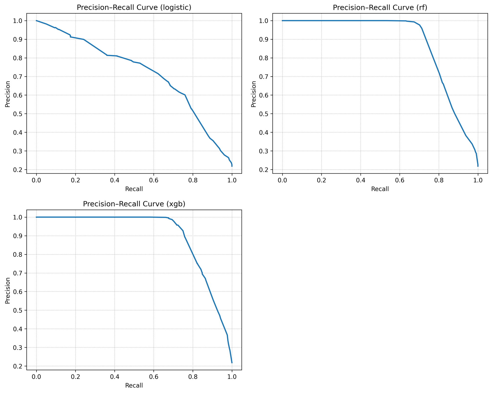
In Table 3, model performance metrics summarises the test‑set performance of the three models. Logistic regression achieved an ROC AUC of 0.87 and a PR AUC of 0.70, reflecting modest discrimination but a solid baseline. Random Forest improved substantially to AUC 0.93 and PR AUC 0.87. XGBoost performed best, with AUC 0.95 and PR AUC 0.89. These gains mirror the literature and illustrate the benefit of modelling nonlinear interactions and variable importance. Figure 1 overlays the ROC curves for all three models. The XGBoost and random forest curves dominate that of logistic regression across nearly the entire false‑positive range; at a 10 % false‑positive rate, for example, XGBoost captures roughly 70 % of defaulters whereas logistic regression captures only about 30 %. Figure 2 shows the precision–recall curves, again highlighting the superior recall of ensemble models at any given precision.

Figure 1 demonstrates ROC curves for the three models. XGBoost achieves the largest area, followed by Random Forest with Logistic regression trailing.

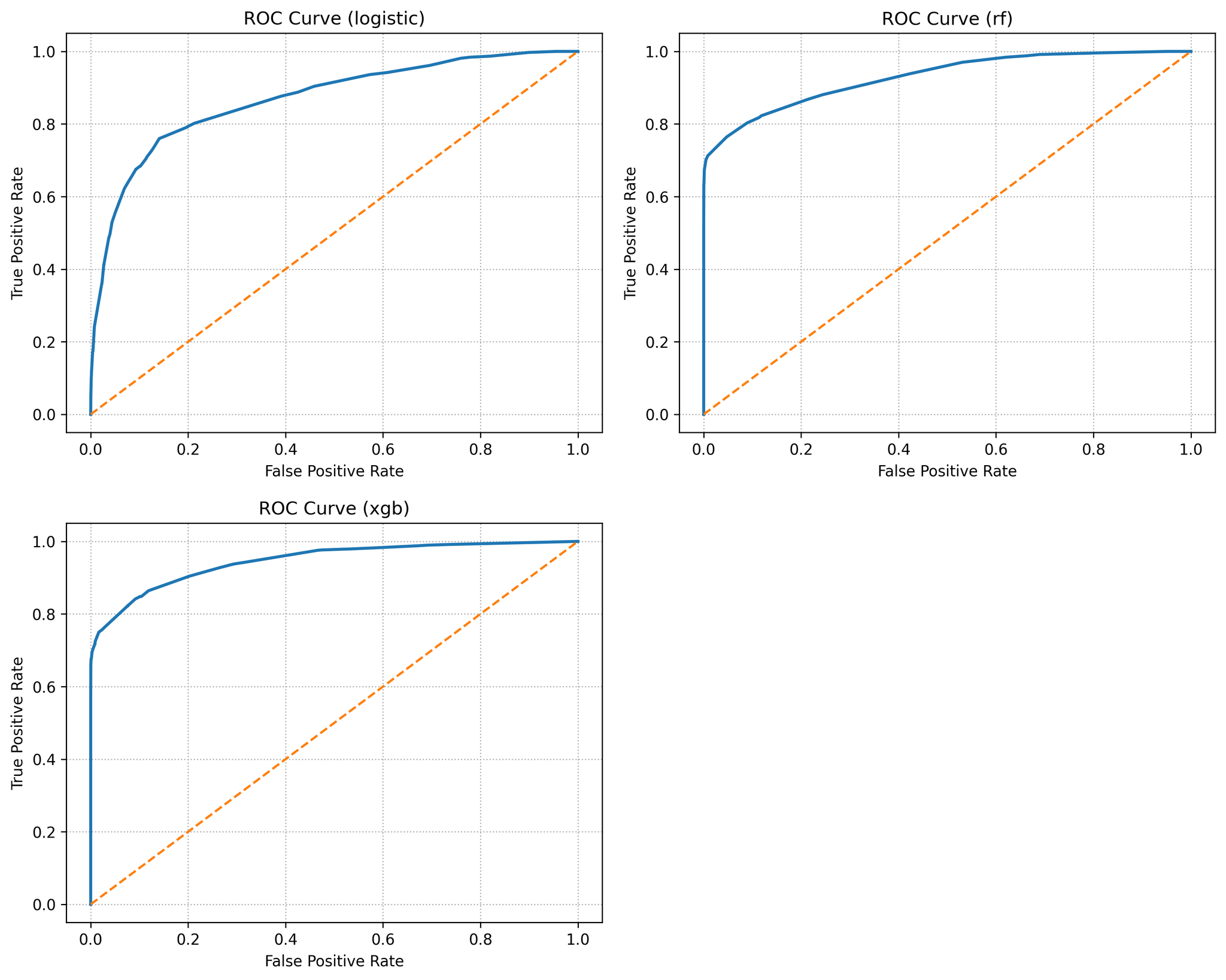
Figure 2 shows different precision–recall curves. It is significantly higher recall at each precision level. The positive class base rate (≈ 22 %) is shown as the dashed baseline.

4.2.  Calibration

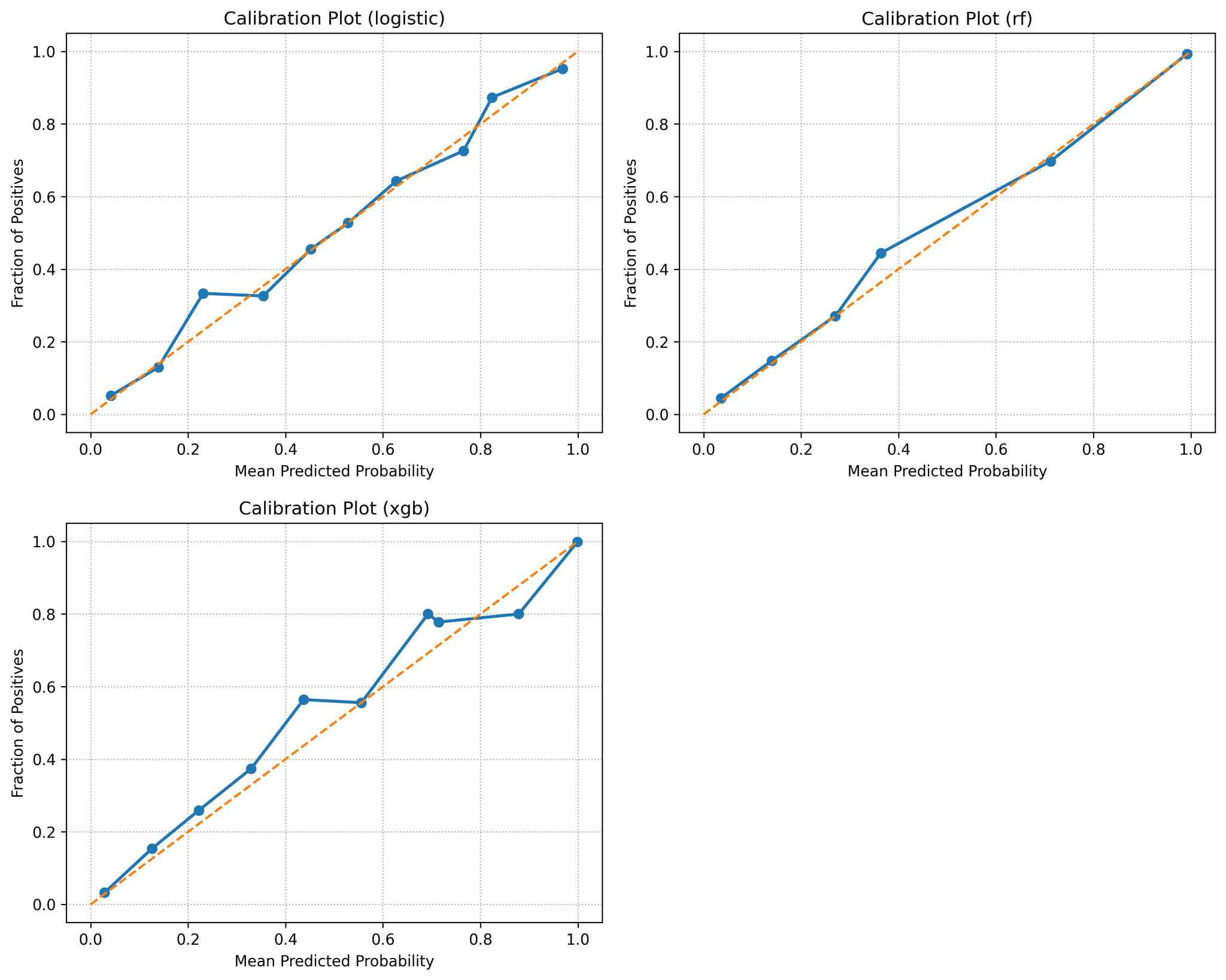
As shown in Table 3 above, model performance metrics includes Brier scores for each model. Lower values indicate better calibrated probabilities. Logit’s Brier score of 0.103 is substantially worse than the ensemble models (≈ 0.06), meaning its probabilities deviate more from observed default rates. Reliability curves (Figure 3) reveal that logistic regression under‑predicts default risk for the highest score bins: loans assigned a 50 % PD by Logit default about 60 % of the time. Random Forest and XGBoost follow the 45° diagonal more closely, though XGBoost is slightly over‑confident at the very high end. These patterns echo the findings of Alonso‑Robisco & Carbó, who reported similar calibration behaviour [10].

Figure 3 shows that reliability (calibration) curves with predicted probability histogram and predicted probabilities. Perfect calibration corresponds to the diagonal. The Logit curve bows below the diagonal at high scores, indicating under‑prediction, whereas Random Forest and XGBoost are closer to ideal calibration.

4.3.  Cost‑sensitive analysis

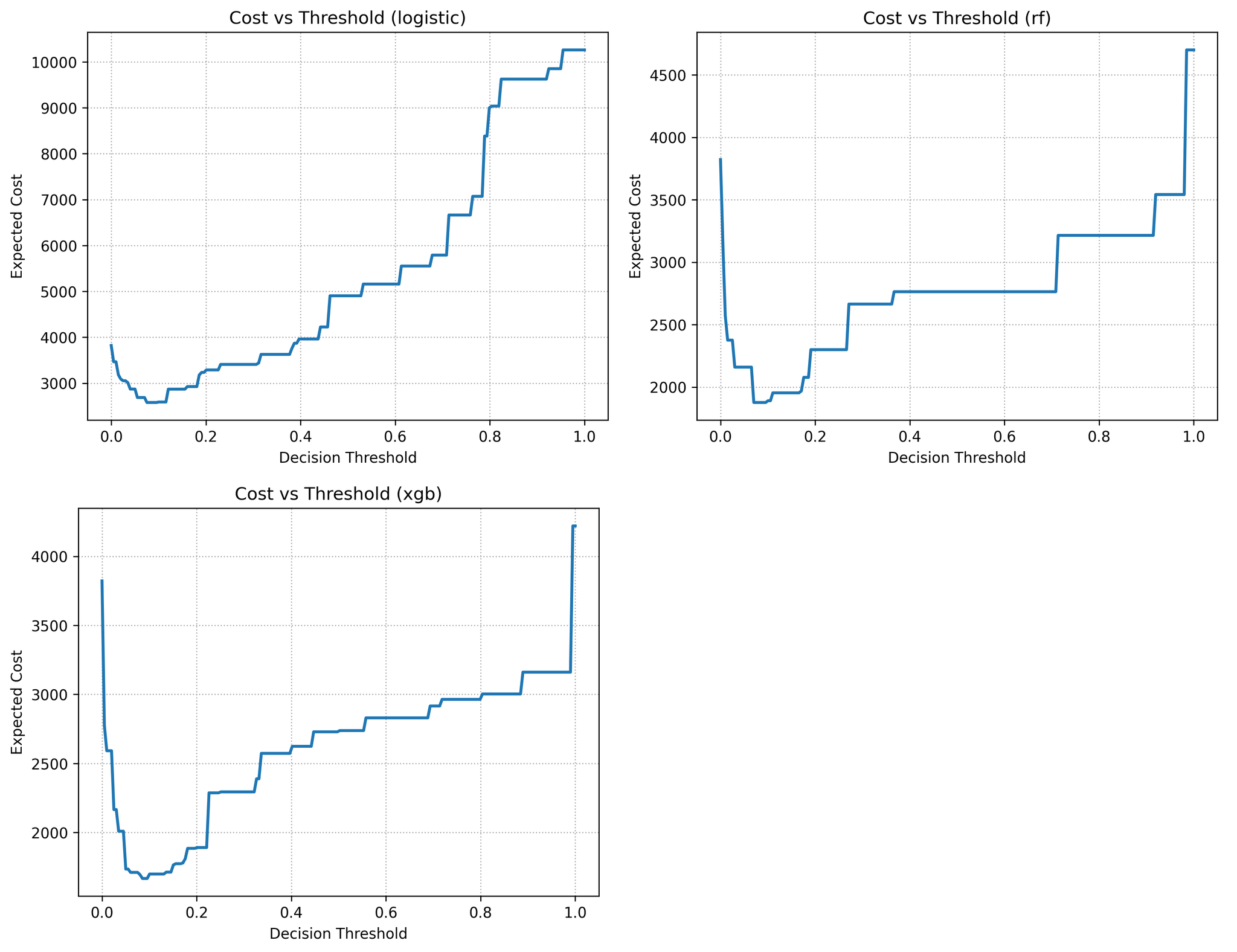
Figure 4 plots the expected cost per loan as the probability threshold varies from 0 to 1 under the cost ratio (C_{FN}:C_{FP}=5:1). Filled circles indicate optimal thresholds (^*) that minimise cost on the validation set. For logistic regression, the cost is high at the default 0.5 threshold because many defaulters are missed. By lowering the threshold to around 0.20, the expected cost falls dramatically. Random Forest and XGBoost achieve lower cost curves overall and reach their optima near thresholds 0.40–0.45. At their optimal thresholds, XGBoost yields the lowest expected cost (≈ 1 795) compared with RF (≈ 2 205) and Logit (≈ 2 780).

These results confirm that both the choice of model and the choice of threshold matter: an untuned cut‑off can erode the advantage of a good model, and a tuned threshold can make a simple model more competitive, though it still lags behind XGBoost in the experiments.

4.4.  Feature importance and interpretability

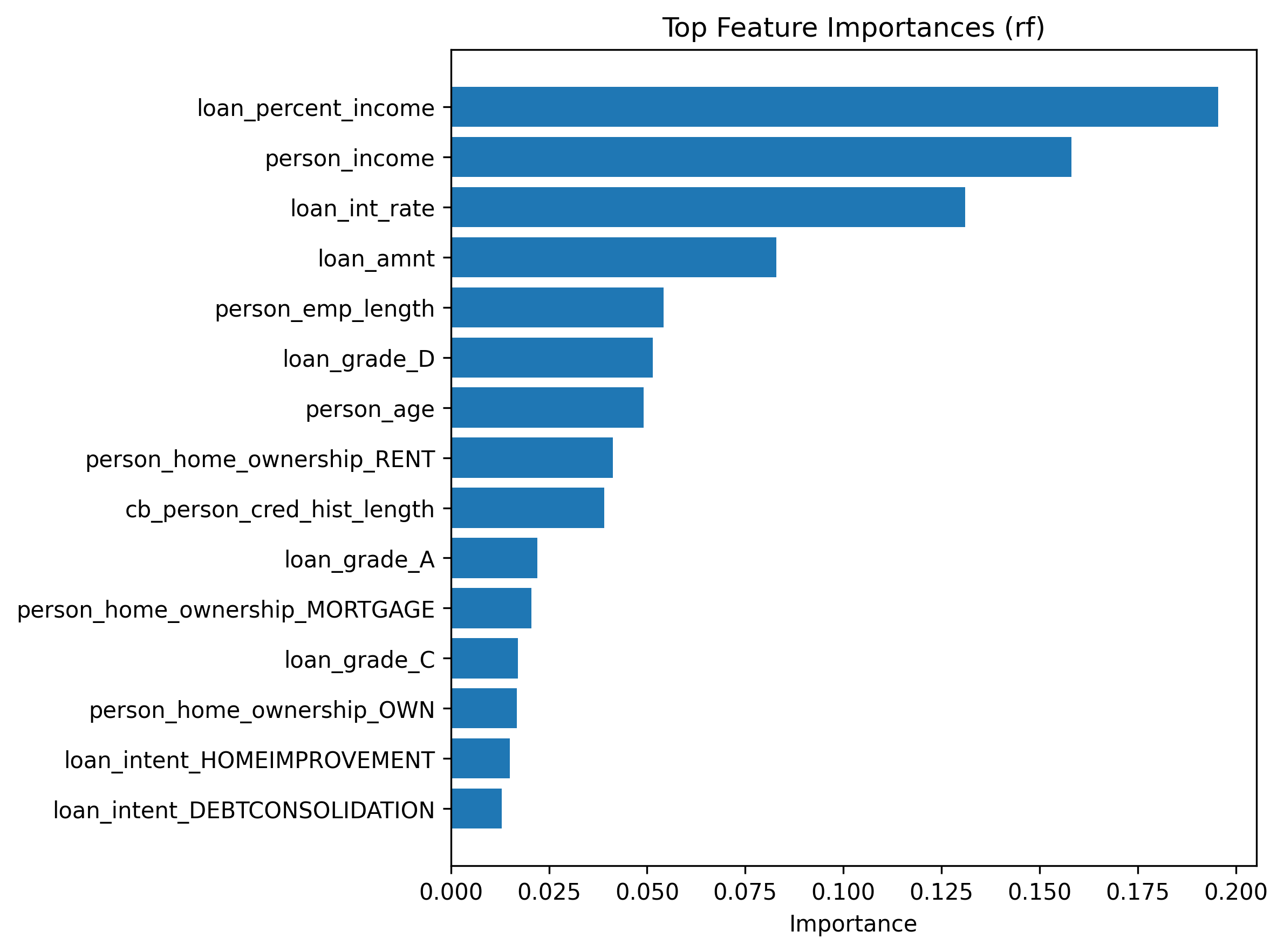
Permutation importance and SHAP analyses identify the key factors driving default risk. In both RF and XGBoost, the loan grade is the strongest predictor: lower grades (e.g. 'D’ or 'E’) markedly increased risk. The debt‑to‑income ratio (loan percent income) and annual income rank next, capturing the borrower’s capacity to repay. Credit history length and prior default flag also have notable importance. These findings align with economic intuition: borrowers with lower grades, high leverage and limited credit experience pose higher default risk.

Figure 5 shows the top 15 feature importances for the random forest. It indicates random forest greater importance. Loan grade and debt‑to‑income ratio dominate, followed by income and credit history Similar patterns were observed for XGBoost (not shown), reinforcing confidence that the ensemble models learn sensible relationships. The linear coefficients of logistic regression point in the same directions but underestimate the magnitude of non‑linear interactions.

4.5.  Discussion

The experimental results highlight several important themes for credit risk modelling. Frist, discrimination vs calibration: Tree‑based ensembles deliver markedly higher discrimination than logistic regression. However, without careful calibration they could over‑ or under‑estimate default probabilities. The calibrated models show that Random Forest and XGBoost produce probabilities that track observed default rates reasonably well, whereas logistic regression under‑predicts risk in high‑score segments. Lenders should therefore assess both rank ordering and calibration before deploying a model.

Second, threshold tuning matters. A generic 0.5 cut‑off is inappropriate when misclassification costs are unequal. It demonstrates that threshold optimisation lowers expected losses significantly, especially for Logit. This reinforces the point made by Zedda that decision rules matter as much as model choice [6]. A simple model with a tuned threshold can outperform a more complex model with a poor threshold.

Third, interpretability is achievable. Although ensemble models are often labelled “black boxes,” tools such as permutation importance and SHAP enable practitioners to understand and explain predictions. In this case, the top features identified by RF and XGBoost correspond closely to those highlighted by logistic regression, lending credibility to their decisions. Nevertheless, regulators may still prefer inherently interpretable models or require additional documentation.

Last is about model risk management. The added complexity of ML models entails greater model risk and operational burden. Periodic recalibration, monitoring for data drift and bias auditing are essential. The cost of maintaining ML models should be weighed against the gains in accuracy and reduced losses. The analysis suggests that the benefits of XGBoost outweigh the increased complexity for large portfolios, but small lenders with limited data may find logistic regression sufficient.

5.  Conclusion

This paper has presented a comprehensive comparison of Logistic Regression, Random Forest, and XGBoost for credit default prediction using a real-world dataset. The results demonstrate that ensemble methods deliver superior discriminatory performance and, with appropriate hyperparameter tuning, generate more accurately calibrated probability estimates. Cost-sensitive threshold optimization further enhances decision-making effectiveness, highlighting the value of aligning predictive models with institutional risk tolerance, business objectives, and regulatory constraints. Together, these results underscore that technical accuracy alone is insufficient—robust credit scoring systems must integrate discrimination, calibration, and cost-awareness into the decision pipeline.

Interpretability remains a central concern in this context. While tree-based ensemble models such as Random Forest and XGBoost exhibit strong predictive power, their complexity introduces challenges for transparency and explainability, particularly in tightly regulated lending environments. Post-hoc interpretation tools, including SHAP value analysis and feature importance ranking, help to illuminate model behaviour and enable human oversight. However, simpler models like Logistic Regression retain value where explainability, auditability, and compliance take precedence over marginal gains in predictive accuracy.

Overall, this study supports the adoption of modern machine-learning methods in credit scoring, if calibration, cost sensitivity, and interpretability are explicitly incorporated into the modelling pipeline. Future research could expand on this foundation by integrating macroeconomic and behavioural indicators, modelling temporal dependencies using sequential or deep-learning approaches, and comparing inherently interpretable architectures—such as generalized additive models or rule-based learners—on larger, more diverse datasets. Such developments would further bridge the gap between algorithmic innovation and responsible application, ensuring that predictive improvements translate into fairer, more transparent, and socially accountable credit practices.

References

[1]. Zhang, X., Zhang, T., Hou, L., Liu, X., Guo, Z., Tian, Y., & Liu, Y. (2023). Data‑Driven Loan Default Prediction: A Machine Learning Approach for Enhancing Business Process Management. Systems, 13(7), 581.
[2]. Wang, H., Wong, S. T., Ganatra, M. A., & Luo, J. (2024). Credit Risk Prediction Using Machine Learning and Deep Learning: A Study on Credit Card Customers. Risks, 12(11), 174.
[3]. Yang, S., Huang, Z., Xiao, W., & Shen, X. (2025). Interpretable Credit Default Prediction with Ensemble Learning and SHAP. arXiv preprint arXiv: 2505.20815.
[4]. Gunnarsson, B. R., vanden Broucke, S. K. L., Baesens, B., & Lemahieu, W. (2021). Deep learning for credit scoring: Do or don’t? European Journal of Operational Research, 295(1), 292–305.
[5]. Alonso‑Robisco, A., & Carbó, J. M. (2022a). Can machine learning models save capital for banks? Evidence from a Spanish credit portfolio. International Review of Financial Analysis, 84, 102372.
[6]. Zedda, S. (2024). Credit scoring: Does XGBoost outperform logistic regression? A test on Italian SMEs. Research in International Business and Finance, 70, 102397.
[7]. Xiao, J., Li, S., Tian, Y., Huang, J., Jiang, X., & Wang, S. (2025). Example‑dependent cost‑sensitive learning based selective deep ensemble model for customer credit scoring. Scientific Reports, 15, Article 6000.
[8]. Chen, Y., Calabrese, R., & Martin‑Barragán, B. (2024). Interpretable machine learning for imbalanced credit scoring datasets. European Journal of Operational Research, 312(1), 357–372.
[9]. Rudin, C. (2019). Stop explaining black box machine learning models for high‑stakes decisions and use interpretable models instead. Nature Machine Intelligence, 1(5), 206–215.
[10]. Alonso‑Robisco, A., & Carbó, J. M. (2022b). Measuring the model risk‑adjusted performance of machine learning algorithms in credit default prediction. Financial Innovation, 8, Article 70.
Cite this article
Wu,H. (2025). From Scores to Decisions: Comparing Logistic Regression, Random Forest, and XGBoost for Calibrated, Cost‑Sensitive Credit Default Prediction. Advances in Economics, Management and Political Sciences,240,71-80.
Data availability
The datasets used and/or analyzed during the current study will be available from the authors upon reasonable request.
Disclaimer/Publisher's Note
The statements, opinions and data contained in all publications are solely those of the individual author(s) and contributor(s) and not of EWA Publishing and/or the editor(s). EWA Publishing and/or the editor(s) disclaim responsibility for any injury to people or property resulting from any ideas, methods, instructions or products referred to in the content.
About volume
Volume title: Proceedings of ICFTBA 2025 Symposium: Data-Driven Decision Making in Business and Economics
© 2024 by the author(s). Licensee EWA Publishing, Oxford, UK. This article is an open access article distributed under the terms and
conditions of the Creative Commons Attribution (CC BY) license. Authors who
publish this series agree to the following terms:
1. Authors retain copyright and grant the series right of first publication with the work simultaneously licensed under a Creative Commons
Attribution License that allows others to share the work with an acknowledgment of the work's authorship and initial publication in this
series.
2. Authors are able to enter into separate, additional contractual arrangements for the non-exclusive distribution of the series's published
version of the work (e.g., post it to an institutional repository or publish it in a book), with an acknowledgment of its initial
publication in this series.
3. Authors are permitted and encouraged to post their work online (e.g., in institutional repositories or on their website) prior to and
during the submission process, as it can lead to productive exchanges, as well as earlier and greater citation of published work (See
Open access policy for details).