1. Introduction

With the rapid development of the Chinese financial market, many scholars and investors seek to invest in the market. Trend following is a popular investment strategy in which you attempt to capture long moves in the financial markets, either up or down. Its simple concept and mechanism make it popular among investors. The Chinese commodity market has long been a target for speculative investors. However, the trading signals cannot be determined precisely in some cases. This study aims to test the feasibility of implementing the MACD trend-following strategy and provides some insights into the subject. This paper organizes a universe to study this strategy methodically. The strategy uses Universe's performance from October 2012 to October 2020 as in-sample data and its performance from October 2020 to August 2022 as out-of-sample data to calculate the portfolio's profit and loss and summarize the difficulties. In light of difficulties, the work includes double Confirmation of MACD and other technical indicators, such as RSI and Bollinger Band, as well as an adjustment of the holding period. As a result, we achieve a positive return with acceptable risks and fluctuations by carefully selecting a combination and holding period. This demonstrates the potential for using a trend-following strategy in the Chinese market. With further research, it is likely to produce efficient investing strategies for the Chinese market.

1.1. Idea

By using the future price to calculate the short-term 12-day exponential moving average and the long-term 26-day exponential moving average and determine the buying and selling signal with the help of the convergence and separation relationship between the two lines, mainly the golden cross and death cross [1].

1.2. Highlight

1.2.1. Strategy Overview

1) Economic Intuition

The goal of the trend following is to use technology that can forecast and identify trends in real-time. Using historical data to predict future trends enables investors to act early and increase profits through the following. Two crosses can reflect the future trend: the golden cross and the death cross. The golden cross occurs when a short-term moving average crosses over a significant long-term moving average to the upside and is viewed by analysts and traders as a harbinger of a definitive market upturn. In contrast, a crossover of the moving averages in the opposite direction produces the death cross and is interpreted to indicate a dramatic market decline. The death cross occurs when the short-term average declines and crosses the long-term average.

2) Signal Generation

The histogram, the difference between the Signal and MACD lines, represents the signal [2]. The signs of three consecutive histograms illustrate the trend and indicate the long or short action.

3) Portfolio Construction

When there is a 'buy' signal for the contract, a long position is executed at the closing price of the next trading day. This strategy trades every three days, and the holding period is three days. To seek a more return and improved hedge, the size of our portfolio is signal weighting.

1.2.2. Performance Estimation

The researcher does the back-testing with data from 2012 to 2020. As the paper mainly focuses on the strategy’s effectiveness in the Chinese Commodity Market, the Wind Commodity Index is used as the benchmark. The annualized return is -0.414%, and the annualized volatility is 14.6%. The Sharpe ratio is 3.05. The MACD trend following strategy applies in the Index. The annualized return is 3.51%, and the annualized volatility is 5.47%. The Sharpe ratio is 0.057. Thus, the strategy is expected to outperform the benchmark. Besides, the low Sharpe ratio means that there is little extra return brought by risk offsets the risk itself, being worth taking risks for more returns. Moreover, the diversified universe is expected to lower the potential risks and seek more profits. So, it is likely that the strategy has a higher Sharpe ratio.

2. Specification

2.1. Qualitative Analysis

Most of an investor's time is devoted to trend analysis and trend-following. The best traders recognize that trend-following drives their decisions, with appropriate parameters in days assisting in analyzing the various trends. The qualitative analysis identifies the various markets that employ technology to generate sufficient profits when trading for various commodities. Traders trade commodities by analyzing market trends critically and ensuring they make the best decisions based on these trends. The analysis of future trends aids in determining whether or not there is a need for investments in trade commodities and how traders make the most prudent investment decisions. In addition, the analysis of contracts using historical trends will aid in financial decisions.

By calculating the difference between the short-term and long-term exponential moving averages, the MACD provides a moving average [3]. The need to calculate the impact of these moving averages on the current prices of the trading instruments is necessitated by the question of which aspects of the trading cycle should be deemed significant. This analysis provides the trader with a clear understanding of the various aspects of the trading cycle and how these aspects can ultimately lead to profits. The investors use the parameters of 12, 9, and 6 days to analyze and forecast the future impact of the trading market on their decisions [4]. Diverse markets also tend to rely on the notion that technology may influence how investors choose to trade their instruments.

2.2. Quantitative Analysis

To analyze the strategy’s performance, The researcher must also calculate Annualized Rate of Return, Annualized Volatility, Yearly Rate of Return, Yearly Volatility, Sharpe Ratio, and Maximum Drawdown Rate using formulas. This strategy's risk-free return for calculating the Sharpe ratio is 3.2%. The bid-ask spread in the paper is the average value for the daily spread.

2.3. Data

2.3.1. Universe

The strategy's universe includes sixteen commodities from four distinct categories: agriculture, metal, chemicals, and energy. The commodities are accessible via the futures exchanges in Shanghai, Dalian, and Zhengzhou. Commodity futures are driven by a standard industry exposure rather than a commodity market component [5]. Thus, our portfolio is varied for hedging several commodities.

Table 1: Commodities varieties.

2.3.2. Data Sets

To follow the trend of future prices, the daily futures price must be known. EMA and MACD indicators can be calculated in the subsequent steps by gathering the data. Moreover, the contract multiplier, tick size, and fee need to be known to calculate transaction costs.

Table 2: The tick size for commodities.

Table 3: The contract multiplier for commodities.

Table 4: The commission fee per lot for commodities.

2.3.3. Data Source

The data are downloaded from Shanghai, Zhengzhou, and Dalian Futures Exchange websites in the form of excel files with a detailed record of daily price, volume, transaction fee, contract multiplier, etc.

2.3.4. Data Range

The data was collected from 2012 to 2022. There will be 80% data for in-sample built-up to guarantee the relative accuracy of optimization. The rest 20% of the data are out-of-sample to evaluate profitability.

2.4. Strategy Detail

2.4.1. Signal Generation

The golden cross and death cross causes the signals generated in the strategy. The sign of the histogram value is H. When \( {H_{t-2}} \) is positive while \( { H_{t}} \) is negative, the histogram changes from positive to negative, indicating the death cross and a downturn in the market trend. Conversely, when \( {H_{t-2}} \) is negative while \( { H_{t}} \) is positive, the histogram changes from negative to positive; it shows the golden cross and an upturn in the market trend.

\( {H_{n}}=\begin{cases} \begin{array}{c} -1,if {H_{n}} \lt 0 \\ 1,if {H_{n}} \gt 0 \end{array} \end{cases}(H=MACD line-Signal line) \) (1)

\( Signal=\begin{cases} \begin{array}{c} -1,if {H_{t-2}} \gt 0 And{ H_{t}} \lt 0 \\ 1,if {H_{t-2}} \lt 0 And { H_{t}} \gt 0 \end{array} \end{cases} \) (2)

The MACD indicator depends on the time constants for the EMAs, which are usually represented as "MACD (12, 26, 9)". Here are the crucial mathematical formulas of the MACD.

1) MACD line: the difference between the short- and long-term exponential moving average (EMA). EMAs of the two different periods can be presented as:

\( EM{A_{t}}({n_{1}})=[\frac{2}{{n_{1}}+1}({P_{t}}-EM{A_{t-1}}({n_{1}}))]+EM{A_{t-1}}({n_{1}}) \) (3)

\( EM{A_{t}}({n_{2}})=[\frac{2}{{n_{2}}+1}({P_{t}}-EM{A_{t-1}}({n_{2}}))]+EM{A_{t-1}}({n_{2}}) \) (4)

Where n1 is the number of days for short-term periods, and n2 is the number for long-term periods.

MACD value is the difference between the fast EMA and the slow EMA:

\( MACD lin{e_{t}}({n_{1}},{n_{2}})=EM{A_{t}}({n_{1}})-EM{A_{t}}({n_{2}}) \)

2) Signal line: an exponential moving average of the MACD line.

\( Signal lin{e_{t}}({n_{3}})=[\frac{2}{{n_{3}}+1}(MACD lin{e_{t}}({n_{1}},{n_{2}})-Signal lin{e_{t-1}}({n_{3}}))+Signal lin{e_{t-1}}({n_{3}})] \)

Where n3 denotes the period for the EMA calculation of the MACDt series.

Only if the histogram values over the most recent three consecutive days change from negative to positive, go long, and vice versa.

2.4.2. Portfolio Construction

\( Trading rules=\begin{cases} \begin{array}{c} long, if Signal=1 \\ short, if Signal=-1 \end{array} \end{cases} \) (5)

When there is a long(short) signal, a long (short) position is executed at the next day's closing price, indicating a one-day lag between the generation of trading signals and the execution of trades. However, if any circumstance other than those listed indicates that our signal is 0, The researcher shall do nothing. Thus, the position is maintained until either a positive or negative signal occurs. If the new signal does not alter, The researcher will re-trade the same position on the trading day. Nevertheless, a reversal trade is conducted if the indication changes direction. Every three days, a signal is generated, so our holding period is three days. The researcher assumes here that our capital base is 1,000,000 RMB. The size of our portfolio is based on signal weighting, which means that the weighting of a commodity today is determined by its return during the preceding three-day period. The weight of each commodity is the three-day return of that item divided by the overall return for the preceding three-day period. This is done to achieve a higher potential return and more effective hedging.

2.4.3. Trade Execution

The transaction costs for commodities contracts in the Chinese market are not high. The researcher trade every three days. The required margin is around 10 to 20 RMB per contract value. The researcher assumes that the cost of a transaction is made up of a commission plus a bid-ask spread of one tick. Effective bid-ask spreads in commodities futures markets are typically smaller than or equal to the amount of one tick per contract [6,7]. Therefore, the researcher calculates transaction cost as a proportion of the notional contract value. Thus, Following, then the researcher can estimate transaction costs TC per lot as below [8]:

\( TC=\frac{(Commission+Tick Size×CM)}{{P_{contract}}×CM} \) (6)

Where CM is the contract multiplier, the number of units of the underlying commodity deliverable per contract; Bid-Ask spread measured in RMB; Price, measured in RMB, is that of the nearby contract at the end of our holding period.

The problem of rolling is significant in the trade execution stage. Futures are traded using a series of contracts that have a brief lifespan and are only active for a few months at a time. The time difference between the contract that is about to expire and the contract that was just formed would cause the back-test and profitability calculations to be skewed. It would also lead to inaccuracies in calculating numerical price indicators, which are the foundation of technical analysis. Therefore, the elimination of gaps in data series is directly related to the resolution of the problem of spliced futures. To get accurate results from our strategy backtesting, the researcher utilizes the 9-days before contract expiry roll technique and the Backward Panama Canal approach [9]. To clarify it, the equation is shown as follows:

\( Roll Differential={P_{new contract}}-{P_{old contract}} \) (7)

\( {P_{adjusted}}={P_{old contract}}+\sum Roll Differentia{l_{t}} \) (8)

Where P is the close price.

3. Implementation

3.1. P&L Graph Cumulative Simple Return (In-Sample)

The cumulative P&L diagram and the summary statistics of the in-sample data (2012-2022) are shown. Although the overall trend is increasing, three decreases are worthy of discussion. The first significant decrease is during the 2014-2015 periods, while the other two less significant periods of negative returns are in 2018 and 2020. In 2018, political friction was responsible for this phenomenon. The United States raised its tariffs on nearly half of its imports from China. China retaliated immediately by imposing tariffs that applied to more than 70% of American goods. That significantly affected China's financial markets. Finally, in 2020, the pandemic negatively affected commodity prices [10].

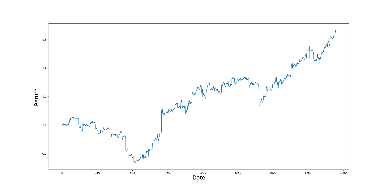
Figure 1: Cumulative return from 2012/10/23 to 2020/10/23 for MACD.

3.2. Statistics and Analysis (In-Sample)

Table 5: Summary statistics from 2012/10/23 to 2020/10/23 for MACD.

The summary statistics show an average result with more than 8% annualized return and 13% annualized volatility. Additionally, the Sharpe Ratio of less than 0.5 indicates that there is still room for improvement.

4. Difficulties

4.1. High Transaction Cost

The holding period for the strategy is three days. The signals are frequently generated because the holding period is short, and many commodities exist in the universe. The high trading frequency leads to high transaction costs, including the loss from the bid-ask spread. At the end of the in-sample period, the transaction cost takes up around one-third of the revenue. As a result, the rate of revenue is 96.2%, and the rate of return is 66.7%.

4.2. Limitation of MACD Indicator

The momentum divergence approach has the opposite issue from the crossover strategy, which restricts being a lagging signal. In particular, it may indicate a reversal too soon, causing the trader to experience a string of minor losses before the major one. The issue arises because a convergent or divergent trend does not necessarily reverse. A market will frequently consolidate for just one or two bars while it takes a breather before regaining strength and continuing its direction. In addition, very little correlation exists between MACD signal strength and generated profit. Investments in financial instruments of any type must be based on multiple indicators [11].

5. Refinement

5.1. Double Confirmation

Combining with another indicator to do the double confirmation can reduce the trading frequency and accurately determine the signal.

5.1.1. RSI

Implementation

The indicator RSI is adopted to double confirm with MACD and lower the trading frequency to avoid high transaction costs simultaneously. RSI indicator measures the magnitudes of recent gains and losses to determine if a stock is overbought or oversold [12]. The oscillator has a range between 0 and 100 and is defined as:

\( RSI=100-[\frac{100}{1+RS}] \) (9)

Where RS= average up index value/average down index value over the seven days.

The commodity is oversold and overbought when the RSI is 30 and 70, respectively. Therefore, a buy signal is created when the RSI crosses over 30, and a sell signal is given when the RSI crosses below 70. A long position is executed only if RSI and MACD give a buy signal and vice versa.

Results

The cumulative P&L diagram and the summary statistics of the refinement to in-sample data (2012-2020) are shown. The overall shape of the diagram is rising upwards. However, the growth is not as sharp as before 2017.

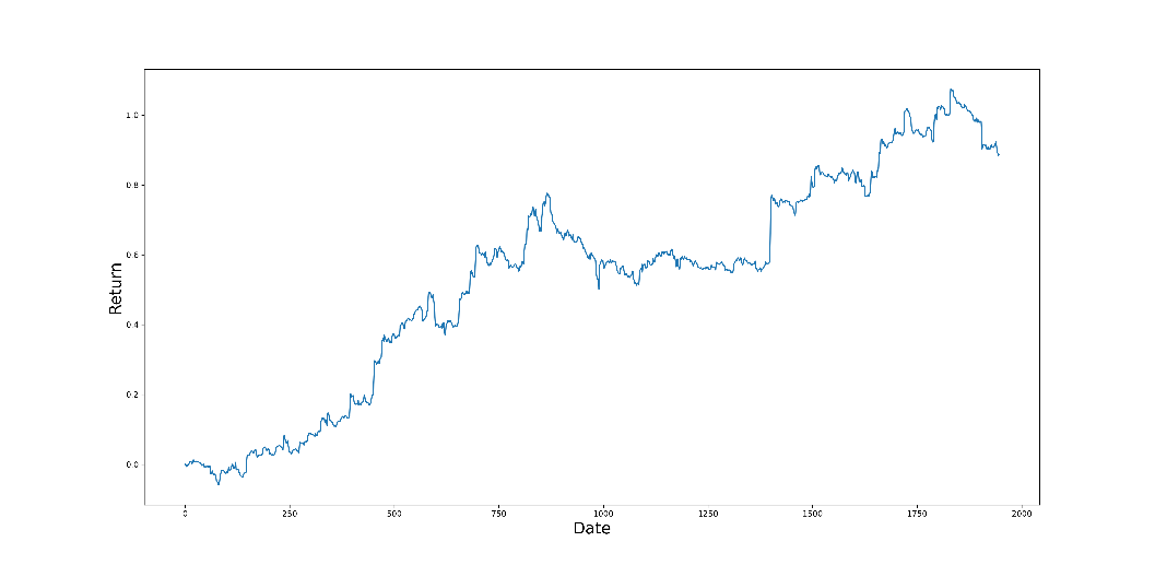
Figure 2: Cumulative return from 2012/10/23 to 2020/10/23 for MACD & RSI.

Table 6: Summary statistics from 2012/10/23 to 2020/10/23 for MACD & RSI.

There are increases in the Sharpe ratio and annualized return and a decrease in the annualized volatility, which means that everything is going on the right track.

5.1.2. Bollinger Band

Implementation

The Bollinger Band methodology, created in the early 1980s, is frequently employed in financial market analysis [13]. Traders widely use Bollinger Bands outputs and other technical indicators to determine which position to take in the asset under observation. The closer prices get to the top band, the more overbought the market becomes, and the closer prices get to the lower band, the more oversold the market becomes.

\( BOLU=MA(TP,20)+m*σ[TP,20], BOLD=MA(TP,20)-m*σ[TP,20] \) (10)

Where BOLU=Upper Bollinger Band, BOLD=Lower Bollinger Band, MA=Moving average, TP(typical price)=(High+Low+Close)/3, m=2(Number of standard deviations), σ[TP,n]=Standard Deviation over last 20-day periods of TP

The buy signal is generated when the futures price moves above the upper band. The sell signal is generated when the futures price moves down to break the lower band. Trades are executed when the Bollinger line and MACD generate a buy or sell signal.

Results

The cumulative P&L diagram and the summary statistics of the in-sample data (2012-2022) are shown. The overall shape of the diagram is rising upwards with tiny fluctuations. It is worth noticing that there was a relatively sharp increase during 2014-2015. Afterward, there was a relatively stable increase from 2015-2018. Then, it turns back to the increment with a high slope. Overall, it is without a doubt that this is a positive trend of cumulative return, and investors should seize the opportunity to consider investing.

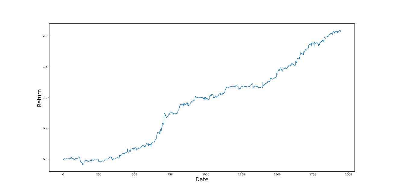
Figure 3: Cumulative return from 2012/10/23 to 2020/10/23 for MACD & Bollinger Band.

Table 7: Summary statistics from 2012/10/23 to 2020/10/23 for MACD & Bollinger Band.

The researcher can see a stable and profitable pattern of the Bollinger Band methodology by analyzing yearly and annualized returns. What is more, the increase in the annualized volatility is limited compared with around a 15% increase in the annualized return. Thus, investors should be optimistic about this excellent and predictable methodology.

5.2. Adjusting Holding Period

5.2.1. Implementation

Another approach to lower the transaction cost is to longer the holding period. The longer the holding period, the number of trading will decrease. Therefore, the different holding period is adopted in two refinement method. The holding periods are 3 days, 6 days, 9 days, 12 days, 15 days, and 18 days.

Result

Table 8: Summary statistics for MACD & RSI in the different holding periods.

Table 9: Summary statistics for MACD & Bollinger Band in the different holding periods.

Putting two tables together gives us a clearer insight into the performances of each methodology. Indeed, the overall annualized volatility of Bollinger Band is higher than that of RSI. However, as long as the researcher considers the massive increase in the annualized return, then it is without a doubt that the strength of Bollinger Band outweighs its limitation. On the other hand, the data of the Sharpe Ratio also represents their performances since Sharpe Ratio considers the risk and return together.

In addition, the researcher can detail the methodology of the Bollinger band by comparing the performances of the different holding periods. An annualized return of 31.361% and a Sharpe Ratio of 1.978 help us identify the 6-day hold period as the best method to enact further.

6. Conclusion

6.1. Final Selection

MACD and Bollinger Band double confirmation with a 6-day holding period is selected. In other words, based on a six-day evaluation, both MACD and Bollinger Band will generate their signals. The trade will not be executed until both indicators generate the same signal. It is evident from the outcomes of implementation and improvement. With a more extended holding period, the trend-following strategy yields a greater annualized return and Sharpe ratio.

6.1.1. P&L Graph Cumulative Simple Return (Out-of-Sample)

The cumulative P&L diagram and the summary statistics of the refinement to out-of-sample data (2020-2022) are shown. The overall shape of the diagram is rising upwards, accompanied by slight variation. However, the increment will slow down after 2022. This is understandable due to the FED's decision to increase interest rates and the overall weak performance of the US market.

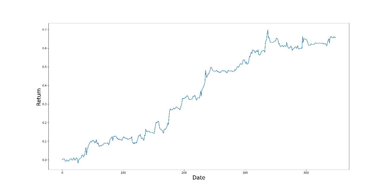
Figure 4: Cumulative return from 2020/10/26 to 2022/8/26 for MACD & Bollinger Band with a 6-day holding period.

6.2. Statistics and Analysis (Out-of-Sample)

Table 10: Summary statistics from 2020/10/26 to 2022/8/26 for MACD & Bollinger Band with a 6-day holding period.

The out-of-sample data shows an ideal result. The annualized return is 32.916%, which is exceptionally high out of our expectations. The annualized volatility is acceptable, which is 16.781%. The sharp ratio of 1.771 also shows a good performance considering risk and return together.

6.3. Additional Consideration

6.3.1. Return

This strategy has delivered very high returns, even reaching 46.996% in 2021. The researcher attributes this phenomenon to high market volatility during the pandemic facilitating technical indicators to generate buy and sell signals. Moreover, as confidence in the stock market has declined during the pandemic, increasing numbers of people are seeking diversion to other markets, such as the futures markets in our study.

6.3.2. Risk

Our Sharpe ratio is 1.77 for 2020-2022. This is supported by an annualized volatility of 16.8 percent and a maximum retracement of 10.9 percent. As a result, our strategy is less speculative. Nevertheless, there are still several risks:

1) Systematic risk: The long-short portfolio hedges a portion of the market risk. Faced with systemic market risk, the portfolio will contain at least one direction of potentially profitable holdings and one partially lost direction. The economy has been undergoing long-term structural reforms, with COVID-19 acting as an internal catalyst to accelerate the change. To hedge risk more effectively, the researcher can apply more economic intuition and qualitative analysis to commodity selection to conduct more research on market trends and execute our selection. Thus, the researcher can significantly mitigate risk by selecting more profitable products. Market risk is primarily based on the fact that market volatility is significantly greater than in the past. There is no assurance that commodity prices will always move in the same direction regarding correlated risk. To mitigate this correlation risk, commodities can be grouped by type, as their prices are more likely to move in the same direction.

2) Leverage risk: Traders can invest as little as 10% of the contract's actual value in futures trading. The leverage magnifies the effect of price fluctuations to the extent that even relatively minor price fluctuations can result in substantial profits or losses. For example, a moderate price decline could result in a margin call or forced position liquidation.

3) Rollover risk: This strategy is affected by the difference between the price at which the old contract expires and the price at which the new contract is executed. Nonetheless, futures contracts frequently trade at a premium or a discount when rolling, resulting in rollover risk.

6.3.3. Correlation

The strategy results are generated from out-of-sample data, significantly since the net investment value is highly correlated with macro markets. The returns are highly related to the inflation of the market. While the strategy can hedge some systemic risks, using a long-short portfolio alone cannot eliminate the risk from impending short-term market shocks.

6.3.4. Operation

The data required for this strategy is published publicly on the websites of each Future Exchange. However, accurate more-frequent data, such as by seconds or minutes, and historical data, such as bid-ask spread, are more challenging to locate. Accessibility is assured, whereas precision is not. In addition, there are two types of usable data: raw data with greater detail and continuous data with less complexity. Processing data is complicated due to the need to deal with the rolling problem and consider insignificant contract-specific details. Moreover, because the portfolio is rebalanced every three days, which is a high frequency, the operational risk may also be high, but it may be purposefully reduced. This strategy's transaction costs could be reduced by extending the holding period.

6.3.5. Future

Trend following strategy is a common strategy used by investors. It is highly crowded and considered to have a low degree of sophistication. However, the method of gaining profit, the weighted approach, and the accuracy of the signals can also distinguish this strategy. In this case, its decay will be slow. It may involve colossal capital, but it cannot be extended to other assets because it exploits the natural characteristics of the commodity. In short, there is still much room for improvement. Nevertheless, it remains a profitable strategy suitable for adoption due to the possibility of efficient markets. In the long term, the researcher believes diversification is critical in designing a robust trend-following strategy [14].

6.3.6. Environment

The strategy is simple, as the operational process and data collection are not complex for investors to handle. The trading frequency is relatively high so that most short-term traders can favor it. The market will still be affected by the current global situation. Essentially, trend following is an intuitive strategy. It should perform well when volatile markets, as they often do in an inflationary environment. History shows that trend following may also perform well after a period of inflation [14].

6.4. Trading Recommendation

Following this strategy, out-of-sample data perform well. The Sharpe ratio exceeds the in-sample data, indicating that the strategy has a low level of risk. In addition, the annualized return is 32.9%, significantly higher than the in-sample return.

In conclusion, it turns out that the strategy is profitable in inefficient markets. China's financial market is not mature yet. Our research will provide valuable insights to investors seeking to profit from this market's apparent inefficiency. Therefore, the researcher advises investors to implement the strategy as soon as possible. The strategy is also easy to manipulate and can generate substantial short-term profits. Even though the MACD indicator has inherent limitations, RSI and Bollinger Band are used in this paper for double confirmation to improve these limitations. In addition, they are adjusting the holding period to find the optimal strategy. This strategy has the potential to become a practical guide for future investors to explore the Chinese market if the MACD parameters are further optimized and the model is enhanced to prevent the occurrence of false signals.

References

[1]. Appel, G. (1979) The Moving Average Convergence Divergence Trading Method, Signalert Corp, 150 Great Neck Rd, Great Neck, NY 11021.
[2]. Chio, Pat Tong. (2022) A Comparative Study of the MACD-Base Trading Strategies: Evidence from the US Stock Market.
[3]. Pedro Nuno Veiga Martins. (2017) Technical analysis in the foreign exchange market: the case of the MACD (Moving Average Convergence Divergence) indicator.
[4]. Kang, Byung-Kook. (2021) Improving MACD Technical Analysis by Optimizing Parameters and Modifying Trading Rules: Evidence from the Japanese Nikkei 225 Futures Market. Journal of Risk and Financial Management 14, no. 1 37. https://doi.org/10.3390/jrfm14010037.
[5]. Chng, Michael T. (2009) Economic Linkages Across Commodity Futures: Hedging and Trading Implications. Journal of banking & finance 33, no. 5: 958–970.
[6]. Followill, R.A., Rodriguez, A.J. (1991) The estimation and determinants of bid-ask spreads in futures markets. Review of Futures Markets 10, 1–11.
[7]. Locke, P.R., Venkatesh, P.C. (1997) Futures market transaction costs. Journal of Futures Markets 17, 229–245.
[8]. Szakmary, Andrew C. (2010) Qian Shen, and Subhash C. Sharma. “Trend-Following Trading Strategies in Commodity Futures: A Re-Examination.” Journal of banking & finance 34, no. 2: 409–426.
[9]. Masteika, Saulius & Rutkauskas, Aleksandras & Alexander, Janes. (2012) Continuous futures data series for backtesting and technical analysis.
[10]. Zhang, D., Hu, M., & Ji, Q. (2020) Financial markets under the global pandemic of COVID-19. Finance research letters, 36, 101528. https://doi.org/10.1016/j.frl.2020.101528
[11]. Halilbegovic, Sanel. (2016) MACD - Analysis of weaknesses of the most powerful technical analysis tool. Independent Journal of Management & Production.
[12]. Wilder, J.W. (1978). New concepts in technical trading systems, Greensboro, NC: Trend Research
[13]. John Bollinger. (2002) Bollinger On Bollinger Bonds, McGraw-Hill.
[14]. Graham Robertson, DPhill. Man Institute. (2022) Gaining Momentum: Where Next for Trend-Following?
Cite this article
Zhu,H.;Li,Y. (2023). The Implementation and Refinement Hedge Fund Strategy in Chinese Commodity Market: MACD Trend Following. Advances in Economics, Management and Political Sciences,12,241-254.
Data availability
The datasets used and/or analyzed during the current study will be available from the authors upon reasonable request.
Disclaimer/Publisher's Note
The statements, opinions and data contained in all publications are solely those of the individual author(s) and contributor(s) and not of EWA Publishing and/or the editor(s). EWA Publishing and/or the editor(s) disclaim responsibility for any injury to people or property resulting from any ideas, methods, instructions or products referred to in the content.
About volume
Volume title: Proceedings of the 2nd International Conference on Business and Policy Studies
© 2024 by the author(s). Licensee EWA Publishing, Oxford, UK. This article is an open access article distributed under the terms and
conditions of the Creative Commons Attribution (CC BY) license. Authors who
publish this series agree to the following terms:
1. Authors retain copyright and grant the series right of first publication with the work simultaneously licensed under a Creative Commons
Attribution License that allows others to share the work with an acknowledgment of the work's authorship and initial publication in this
series.
2. Authors are able to enter into separate, additional contractual arrangements for the non-exclusive distribution of the series's published
version of the work (e.g., post it to an institutional repository or publish it in a book), with an acknowledgment of its initial
publication in this series.
3. Authors are permitted and encouraged to post their work online (e.g., in institutional repositories or on their website) prior to and
during the submission process, as it can lead to productive exchanges, as well as earlier and greater citation of published work (See
Open access policy for details).