1. Introduction

The financial markets are usually unpredictable and full of uncertainties. Investment risk is a significant concern in the financial markets [1]. And it is strongly related to the market laws of itself and contingencies. National policies, natural disasters, and economic crises will impact the financial market and the return on investment. As a result, the investors hope to find approaches to hinder investment risks and improve returns simultaneously.

As ordinary people urgently need reasonable wealth distribution theory, learning to optimize investment and financial management and achieve sound investment is the most concerned issue for investors.

For investors, the investment goals typically are maximizing returns under given risks, and different people perceive various risk preferences or just maximizing the cumulative returns during the investment period. Risks and returns are constantly coming together; the most crucial part of investment optimization is to find the optimal allocation of existing wealth resources among risky investable assets within a given risk preference.

Regarding portfolio optimization, one of the essential subjects of modern finance is to investigate how to rationally and reasonably purchase/allocate financial products in an uncertain environment to achieve a desired equilibrium between yield and risk [2].

In financial history, portfolio theory is also called diversification investment theory [3,4]. As its name indicates, diversification does not put all eggs in the same basket; it investigates the best way for investors to distribute available funds when funds are restricted and expected returns are undermined. Thereby avoiding the risks in the financial market and maximizing returns.

Another way to understand investment is to exchange risk compensation (income) by assuming certain risks. Generally speaking, with greater risk, the return will be improved. Hence, the compromise between risk and return must be accepted when investors make investment decisions based on their circumstances.

To realize the optimization of investment, quantifying the investment is usually a must, which can be done in the quantitative investment field. Quantitative investment takes advantage of computer science techniques and specific mathematical algorithms to evaluate investment ideas and realize investment strategies [5]. In essence, quantitative investment is to observe the laws and study the pattern of markets, then attempt to discover the relationship between various factors that could help to determine future stock price returns.

2. Stock Dataset

The dataset of different stocks is obtained from the Python finance package. In this report, 27 stocks are selected from 2010/01/02 to 2023/03/11 since not all the tickers are valid in this experiment. The chosen 27 stocks are EOG Resources, Occidental Petroleum, Enbridge, NextEra-Energy, Enterprise Products, Delta Air Lines, Biglari Holdings, Danaher Corporation, Paccar, Walmart, Procter \& Gamble, Coca-Cola Company, Pepsi, Costco, Bank of America, Morgan Stanley, Unum, Progressive, Master Card, Apple, Microsoft, Visa, Google, IBM, Netflix, Visteon, Verizon.

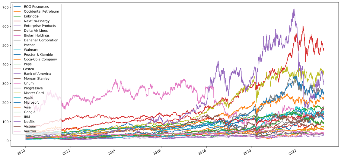
Figure 1: 27 stocks’ price trends from 2010/01/02 to 2023/03/11.

The overall trends of all the stocks are shown in Figure 1, it can be observed that the general direction is almost the same, and in some critical time, for example, in 2019 and around 2021, due to Covid, basically all the stocks go down drastically at the same time.

2.1. Calculate the Daily Rate of Return for a Stock

Calculate the stock's return daily, and the corresponding return curve. The daily return of a stock is given by percentage change, it can be observed that around 2020, the minimal return occurs. Back to the prices curve, the price goes down drastically. The most stable prices curve 'Unum' is also stable in the return curve.

3. K-means for Choosing Five Stocks

There are 27 stocks; however, instead of clustering the stocks based on different industries, we explore this dataset from the data perspective. The k-means clustering is utilized to classify the company into five groups. Then calculate the mean return of each stock as shown in Table 2

Table 1: The average return on 27 stocks.

In Table 2, all the mean returns are positive. And the largest returns happen in "Netflix" and "Apple," which are quite similar. The k-means algorithm is universal, and here we mainly employ such a method rather than study it; the Principal Component Analysis is used to reduce the dimension of each stock return data into two dimensions for visualization. Then, the K-means clustering method is responsible for clustering the 2-dimensional data into the desired number of groups based on Euclidean distance [6]. In the PCA procedure, the time series value of each stock is processed based on the following steps: Standardization is critical to perform standardization before PCA since it's sensitive regarding variances of the initial variable. Compute the covariance matrix to evaluate how much deviation or how many relationships between two variables. Obtain the eigenvalues and eigenvectors of the covariance matrix to determine the principal components of the data by ordering the percentage of explained variances.

Table 2: K-means results for five groups with maximizing mean returns.

The selected five groups are 'Costco,' 'Netflix,' 'Visteon,' 'Occidental Petroleum,' 'And Microsoft’ In Figure 2, reduced data are arranged in the black dot, and the centroids are depicted as a white cross; different groups are shown with different colors.

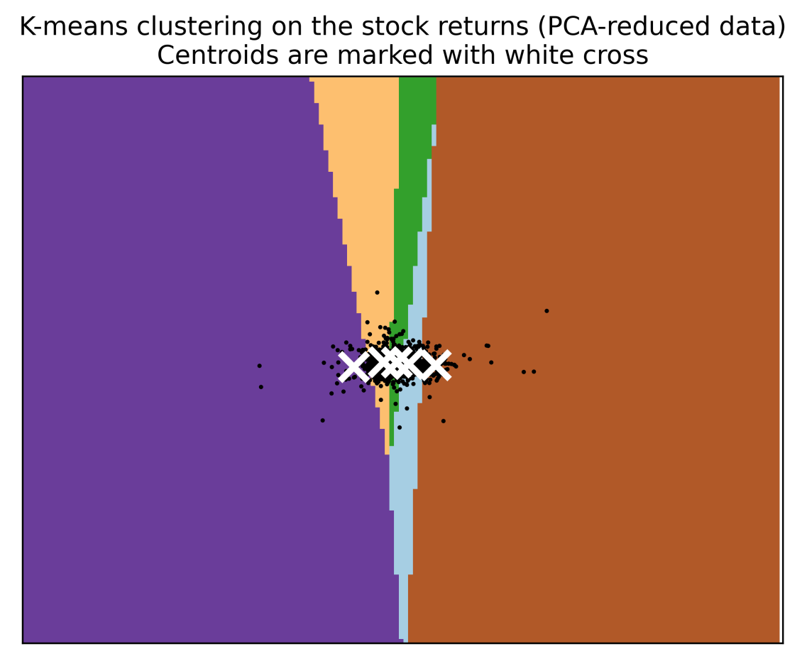
Figure 2: K-means clustering on five groups from 27 stocks.

With the k-means clustering on five groups, choose the maximum mean return in each group, as shown in Table 2.

4. Portfolio Return Calculation

We have selected 5 stocks, and the number of preferred stocks is fixed. Next, we should consider how we can allocate resources with unknown weights.

In this section, the portfolio return can be obtained by summating different stocks with weights. First, we can get an initial return with random consequences to check how the portfolio performs.

4.1. Portfolio with a Given Weight

As explained before, the primary choice is to a set of weights manually, with the summation of each value as unity. The weights corresponding to 5 individual stocks are 'Costco': 0.32, 'Netflix':0.15, 'Visteon':0.10, 'Occidental Petroleum':0.18, and 'Microsoft': 0.25. Incoming supplies are multiplied by their calculated weight to obtain weighted stock return value; then, the summation of the weighted income of five stocks is to get the payment of the portfolio investment.

In this program, the cumulative return curve drawing function cumulative_returns_plot() can be defined, and the cumulative return curve of a given weight portfolio can be drawn.

4.2. Equally Weighted Portfolio

The second solution is to evenly distribute the weight of each stock so that they are all equal. This is the easiest way to invest and can be used as a benchmark for other portfolios. The same calculation method can be conducted with values of 0.2 for each stock.

4.3. Market Value-weighted Portfolio

This section will study the portfolio with the weighted market value of the stock. In other words, stocks with higher market value correspond to greater weights, which are proportional to the market shares. When these stocks perform well, the portfolio's performance will also improve.

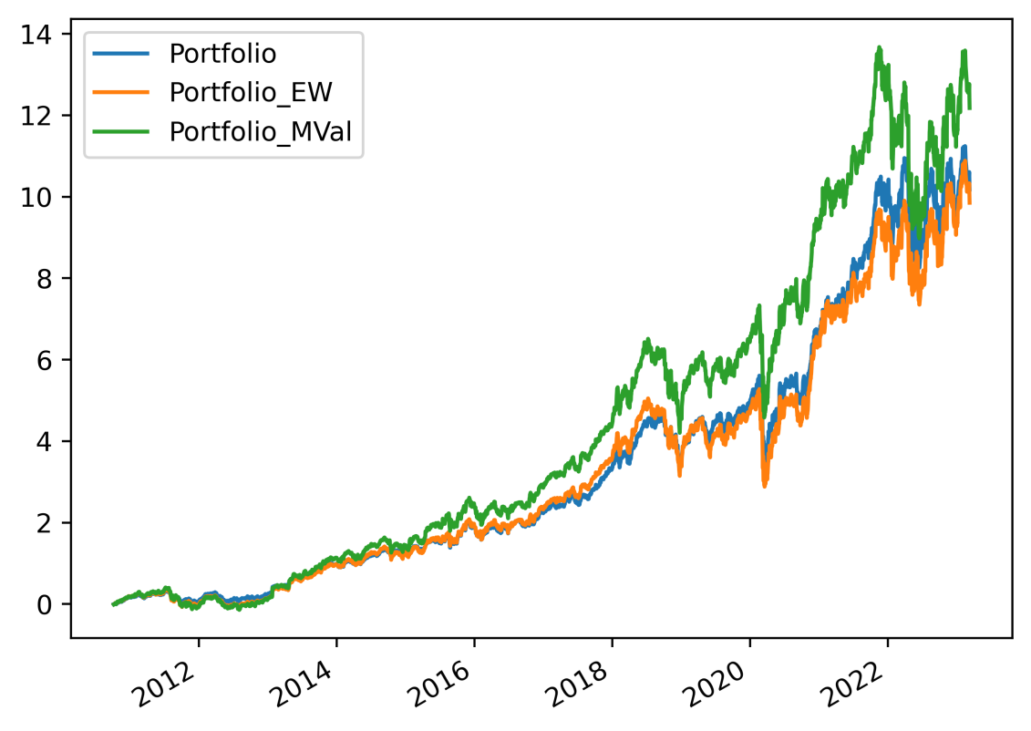
Figure 3: Portfolio returns on the market value-weighted portfolio.

5. Portfolio Correlation Analysis

5.1. Portfolio Correlation Matrix

We can utilize the correlation matrix to get the approximated linear correlation between multiple stock price returns. In the Python Pandas package, this can be achieved by simply using the corr() method.

Each entry in this matrix is the correlation coefficient of two selected stocks, ranging from -1 to 1. It can be observed that the diagonal entries of the matrix are always one since the correlation of one store and itself is, of course, perfectly correlated. Furthermore, the correlation matrix is symmetrical. Thanks to the Python package seaborn, the numerical correlation matrix can be displayed as a heat map for observation.

It can be found that the most significant correlation happened in stock 'Costco' and stock 'Microsoft.' On the other hand, since the original 27 stocks are processed with PCA as well as k-means, in other words, the similarity between the two stores in the different clusters has been reduced before. As a result, it can explain that the correlation between the selected five stocks is generally not high.

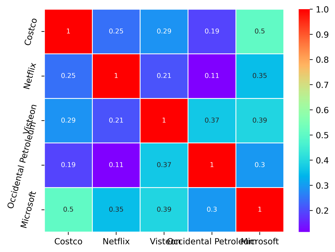
Figure 4: Portfolio Correlation Matrix.

5.2. Portfolio Covariance Matrix

Compared with the correlation coefficient, which may only reflect the linear relationship between two stocks. The covariance matrix contains more information about the uncertainties to inform us of the volatility of the stocks.

The built-in function .cov() can be used in Python to get the covariance matrix for a given pandas DataFrame.

5.3. Portfolio Standard Deviation

The standard deviation, the square root of the variance, is normally used to quantify volatility and portfolio risk. There are some disputes about which quantity is the best to evaluate the risk. However, variance is the most convenient one, and the risk can be estimated by

\( σ=\sqrt[]{(wt\sum w)}\ \ \ (1) \)

σ, the standard deviation of the portfolio

6. Explore the Optimal Portfolio of Stocks

What kind of combination weight should be chosen is the best? Is it to maximize profits? Or the least risky? We need to weigh the two factors of risk and benefit comprehensively. The portfolio theory proposed by Markowitz, a Nobel laureate in the research field of economics, is popularly applied in portfolio selection and asset allocation. The mean-variance analysis method and efficient frontier model in this theory would be used to find the optimal investment portfolio.

6.1. Simulate the Markowitz Model Using Monte Carlo

Mean-Variance Model in modern portfolio theory, also known as the mean-variance model, was proposed by Harry Markowitz [7]. It's a mathematical model to evaluate a portfolio of assets to maximize the expected return.

The essential idea is to diversify the investment; for an investor, the portfolio risk can simply be reduced by holding combinations of different assets that are not perfectly correlated. It is the diversification that guarantees the same expected return while keeping the risk at a low level.

In the mean-variance analysis, the calculation of the mean and variance of individual assets and the portfolio will be studied. For example, one can compare which investments have the most significant expected returns and lowest variance. Suppose an investor decides to purchase two different investment portfolios: he first buys asset A with $300,000, whose return rate is 10%. The other investment B, with the amount $300,000, whose expected return rate is 10%. Since he decides to purchase the portfolio with $400,000, the weight of each asset can be obtained based on the buying amount; as a result, for assets A, the weight is 0.75, and for Investment B, the weight is 0.25. Furthermore, the total expected return of this portfolio can be calculated simply with the weighted sum, which gives us the expected return of this portfolio is 8.75%.

On the other hand, the variance of our portfolio is much more complex.

It cannot be the weighted summation of the two investment's clashes; since a correlation exists between the two investments, other conflicts will be added. Suppose, in this case, the correlation of the two assets is 0.5, and the standard deviation of investments A and B are 0.14, 0.07, respectively. the variance of this portfolio is

\( {σ^{2}}=(25{\%^{2}}*7{\%^{2}})+(75{\%^{2}}*14{\%^{2}})+（2*25\%**75\%*7\%*14\%*0.65）=0.0137\ \ \ (2) \)

the standard deviation = 0.1171, If the asset pairs correlate 0, the portfolio's risk takes the lowest value; if the asset pairs correlate 1, it can give the highest possible standard deviation of portfolio return.

As a result, it will be less risky than owning one type of financial asset.

The risk is measured by variance. What mean-variance analysis provides investors is the insight to find the most significant return at a particular risk. Or, on the contrary, to find the slightest chance at a given level of return based on different investment preferences.

For a portfolio (take three financial assets A, B, C as an example), the expected returns can be obtained with

\( E({R_{p}})={w_{A}}E({R_{A}})+{w_{B}}E({R_{B}})+{w_{C}}E({R_{C}})\ \ \ (3) \)

on the other hand, the variance of the portfolio is

\( σ_{p}^{2}=w_{A}^{2}σ_{A}^{2}+w_{B}^{2}σ_{B}^{2}+w_{C}^{2}σ_{C}^{2}+2{w_{A}}{w_{B}}{σ_{A}}{σ_{B}}{ρ_{AB}}+2{w_{A}}{w_{C}}{σ_{A}}{σ_{C}}{ρ_{AC}}+2{w_{B}}{w_{C}}{σ_{B}}{σ_{C}}{ρ_{E}}\ \ \ (4) \)

Monte Carlo simulation is used for analysis; that is, a collection of weights is randomly generated, the income and standard deviation of the combination are calculated, and this procedure is repeated many times (for example, 10,000 times) [8]. The income and standard deviation of each combination is calculated. Plotted as a scatterplot.

The basic philosophy for investment is to find the balance between risk and return. Figure 5 depicts all the possible outcomes. Each point represents a portfolio case; the x-axis represents the standard deviation of risk, and the y-axis represents the return rate. According to Markowitz's portfolio theory, a rational investor consistently maximizes the expected return at a given level of risk or minimizes the expected risk at a given level of return. Reflected in the figure is the efficient frontier around the boundary. Only the points on the efficient frontier are the most efficient portfolios. We now know rational investors will choose portfolios on the efficient frontier, the top with minimal x value. Under this consideration, there are some strategies one may reckon on [9].

6.2. Portfolio with Minimal Investment Risk

One strategy is to choose the minimum risk portfolio (GMV portfolio). The word GMV comes from the global minimum variance. In Figure 5, the red dot represents the GMV portfolio, and in this case, the corresponding weights are Costco:0.6633156, Netflix:0.07523087, Visteon: 0.04465153, Occidental Petroleum: 0.0942384, Microsoft: 0.1225636.

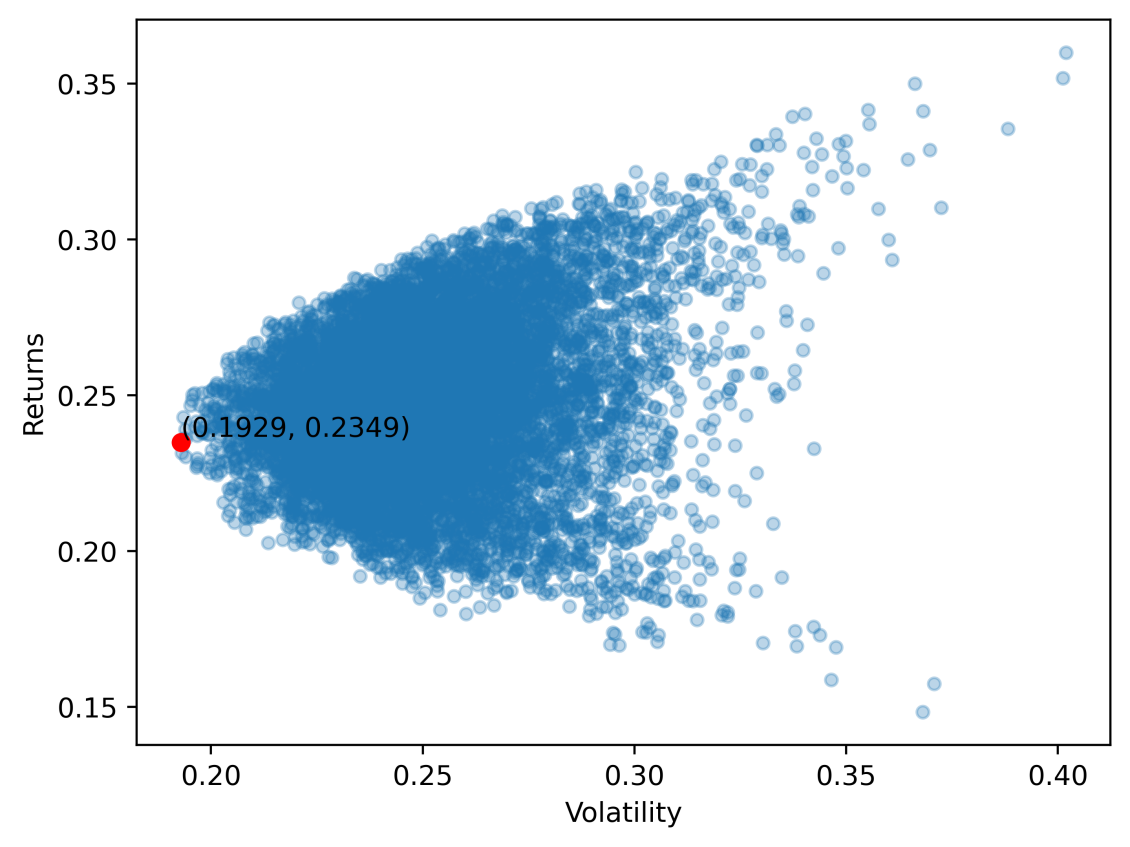
Figure 5: Portfolio with minimal investment risk.

Calculated weights to achieve minimum risk portfolio are as follows, 'Costco':0.6633156, 'Netflix':0.07523087, 'Visteon':0.04465153, 'Occidental Petroleum': 0.0942384, 'Microsoft': 0.1225636. And the resulting portfolio curve is shown in Figure 6. the blue line refers to the initial portfolio; in this case, the portfolio returns are the baseline. The orange line refers to the equally weighted portfolio. The green line has the highest portfolio return since its' weights were based on market values; in this case, the risk is out of consideration. Finally, the red line demonstrates the GMV method; the return is not high since the potential risk is a significant consideration.

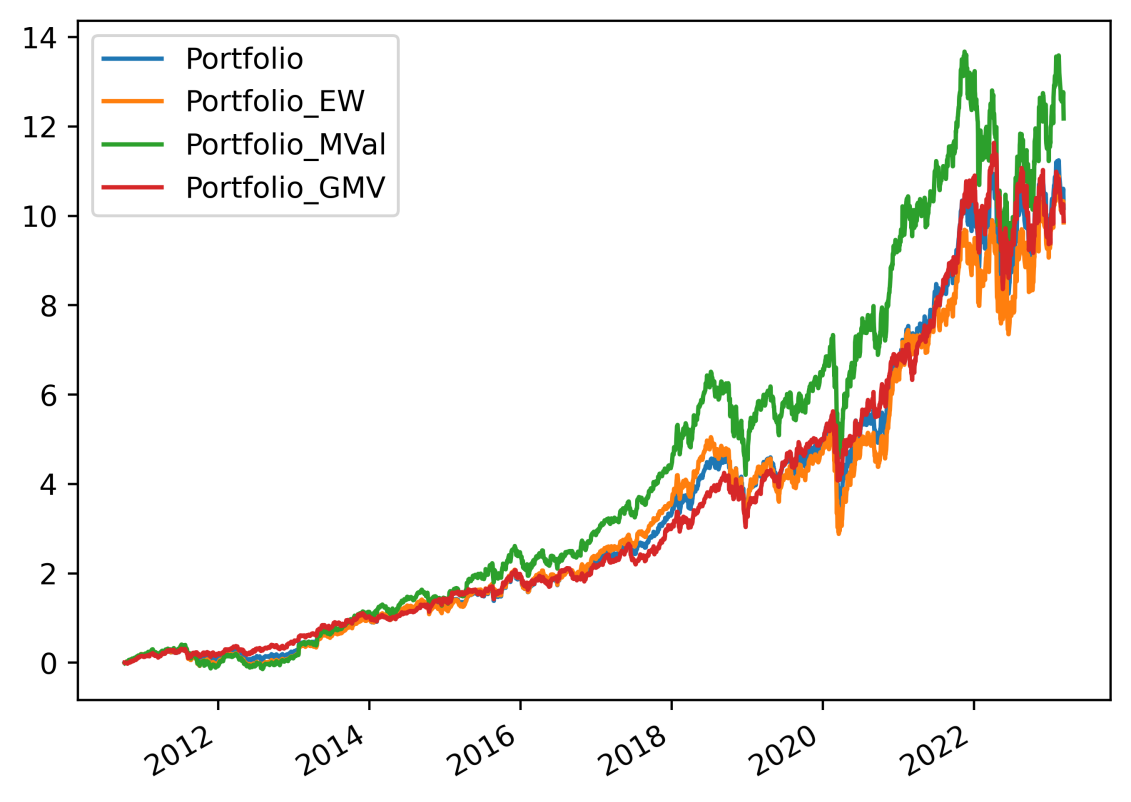
Figure 6: Portfolio Returns (red) with minimal investment risk.

6.3. Invest in the Best Portfolio

Nobel laureate William Sharp proposed Sharpe Ratio to help investors compare investment returns and risks [10,11]. Rational investors generally fix the trouble they can bear and pursue the maximum return; or improve the expected return and seek the minimum bet. So the Sharpe ratio calculates the excess return per unit of total risk taken. Calculated as follows:

\( SharpeRatio=\frac{{R_{p}}-{R_{f}}}{{σ_{p}}}\ \ \ (5) \)

R_p return of the portfolio

R_f risk-free rate

\( {σ_{p}} \) standard deviation of the portfolio's excess

The numerator calculates the delta, the excess return on investment compared to a benchmark representative of the entire investment class. Standard deviation $\sigma_{p}$ of the denominator refers to the volatility of the return, which agrees with risk. Since the higher volatility is equivalent to higher risk, next, simply divide the mean of excess returns by its standard deviation to get the Sharpe ratio, which measures return over the stake. In addition, the annualized Sharpe ratio can be obtained by multiplying with \( \sqrt[]{252} \) (252 refers to the trading days in one year)

\( AnnualizedSharpeRatio=\sqrt[]{252}*\frac{{R_{p}}-{R_{f}}}{{σ_{p}}}\ \ \ （6） \)

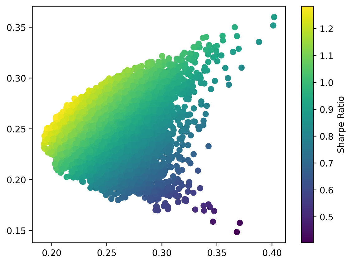
Figure 7: Portfolio Sharpe ratio.

Selection of Optimal Sharpe Ratio Combination is what we desire to discover a so-called optimal balance between returns and risks. It's the Sharpe ratio that can assist us in conducting more clear analysis. The Sharpe ratio gives us the excess return generated by each unit of risk. The first step is to evaluate the Sharpe ratio equivalent to the fusion of the above Monte Carlo simulation and plot it as the third variable in the return-risk scatter plot. Here, the visual clue of color is used to represent the Sharpe ratio. It can be observed that there exists an edge for the high Sharpe ratio; in this region, we also would like to find out the apex of such a convex shape and the resulting Figure 8.

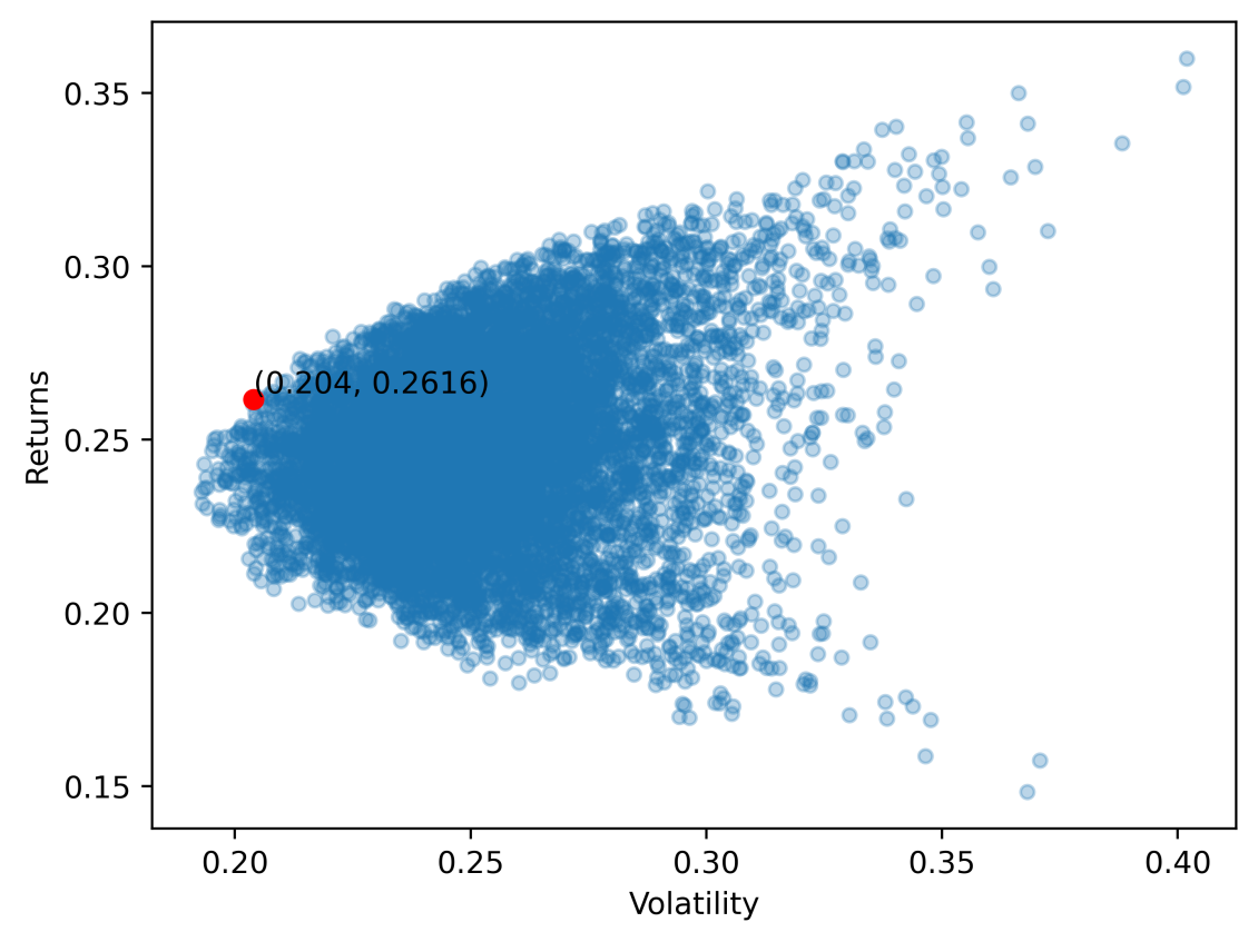
Figure 8: Selection of sharpe optimal combination.

There are some important for using the Sharpe ratio; the Sharpe ratio can be used to evaluate a portfolio's risk-adjusted performance. To explain if the excess returns of a given portfolio will be responsible for the wise investment or just random luck. However, it's not the metric for us to consider the Sharpe ratio as the "best" portfolio option here from a theoretical perspective.

We find that the combinations along the upper edge of the scatterplot have larger Sharpe ratios. Then observe the mixture with the highest Sharpe ratio and draw it on the return-risk scatter diagram. Sharpe Ratio grading thresholds have four levels: when less than 1, defined as bad, and when the ratio is from 1 to 2, we can regard it as adequate or just suitable since the excess return is just more significant than the variance, while when Sharpe ratio is more extensive than two and less than 3, this is much more favorable, when extensive than 4, it would be excellent, and it might happen some cases.

To achieve the maximum Sharpe ratio of the portfolio, the following weights of five stocks can be used, 'Costco': 48694022, 'Netflix': 0.13380845, 'Visteon': 0.00482005, 'Occidental Petroleum': 0.03527024, 'Microsoft': 0.33916104. The returns are generally hard to predict, while the volatilities (standard deviation) and correlation tend to be more stable. So, we first consider to minimizes the standard deviation. The GMV portfolio often outperforms the MSR portfolios out of sample, while the MSR performs better for in-sample. In actual investment, out-of-sample results are more crucial for us.

On the other hand, The MSR portfolio is popular in theory since it has a high historical Sharpe ratio. Still, it can't guarantee that the portfolio will continue to have a good Sharpe ratio. In conclusion, the GMV portfolio result is much more valuable for investment.

Even though the above discussions only contain stocks for our analysis, the essential idea remains for more complex combinations. In an investment portfolio, various financial assets such as shares, futures, ETFs, options, and derivatives will be held. The underlying risk/return level for individual security will strongly affect the Sharpe ratio. And with diversification, stocks, shares, and other financial instruments are combined to hedge. Suppose a hedge fund manager has a portfolio of stocks (similar to what we discuss in the above sections), and the Sharpe ratio is 1.70. He added some commodities to diversify the allocation with a rate of 0.8/0.2 for stock/items. As a result, the Sharpe ratio is pushed up to 1.9.

In this case, although adjusting this portfolio would generally enhance the risk level, it pushes the ratio up, resulting in a more preferable risk/reward circumstance; it's common for us to achieve such a high ratio. On the other hand, when the change of a portfolio leads the balance to improve, the portfolio addition, at the same time, potentially offers attractive returns.

In some sense, many financial analysts will evaluate the Sharpe ratio when hitting a much more unacceptable risk level, then decide not to change the portfolio.

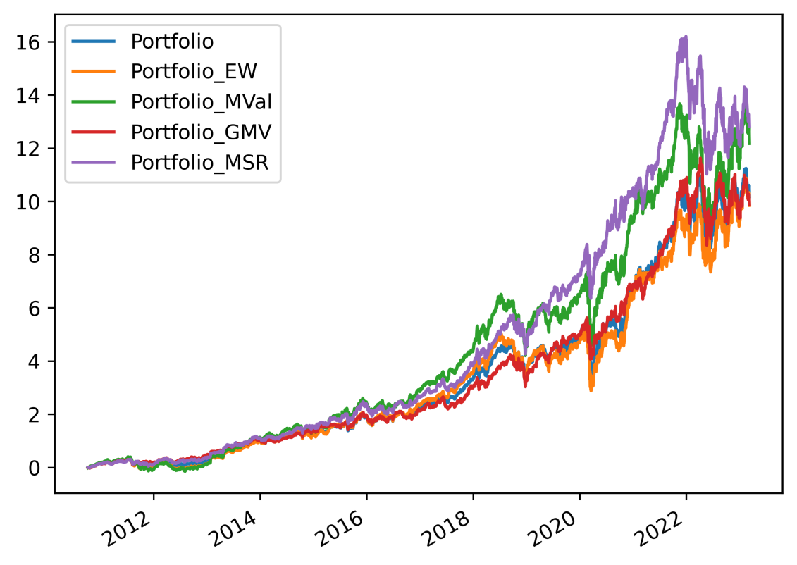
Figure 9: Portfolio Returns (purple) on selection of Sharpe Optimal Combination.

7. Conclusion

In this report, the quantitative analysis of financial time series from the US stock markets involved clustering the returns of all stocks using the K-means algorithm with five centroids. Within each cluster, the store with the maximum return was selected. The selected five stocks were then used to construct a portfolio with different stock weights. The combination was optimized using Monte Carlo simulation while considering risk mitigation and maximizing the Sharpe ratio. The results revealed that maximizing the Sharpe ratio scenario could achieve the optimal portfolio. Additionally, the weights based on market value also presented remarkable cumulative returns.

Furthermore, plans also include incorporating more evaluation metrics to assess the performance of the optimized portfolio. These metrics could include downside risk, value at risk (VaR), and maximum drawdown. Additionally, incorporating factors such as company size, industry, and financial ratios could further improve the accuracy of the portfolio optimization approach.

Future efforts in this area will focus on expanding the analysis to consider more stocks and clusters. The aim is to improve the accuracy of the portfolio optimization algorithm and further explore the possibilities of mitigating risk while maximizing returns. Moreover, the study seeks to investigate the applicability of this approach in alternative markets and asset types. By doing so, the research will contribute to developing a comprehensive portfolio optimization strategy for investors.

References

[1]. Pagano, Marco. "Financial markets and growth: An overview." European economic review 37.2-3 (1993): 613-622.
[2]. Black, F., & Litterman, R. (1992). Global portfolio optimization. Financial Analysts Journal, 48(5), 28–43. https://doi.org/10.2469/faj.v48.n5.28
[3]. Jorion, Philippe. "Portfolio optimization in practice." Financial analysts journal 48.1 (1992): 68-74.
[4]. Perold, Andre F. "Large-scale portfolio optimization." Management Science 30.10 (1984): 1143-1160.
[5]. DeFusco, Richard A., et al. Quantitative investment analysis. John Wiley & Sons, 2015.
[6]. Tola, Vincenzo, et al. "Cluster analysis for portfolio optimization." Journal of Economic Dynamics and Control 32.1 (2008): 235-258.
[7]. Steinbach, Marc C. "Markowitz revisited: Mean-variance models in financial portfolio analysis." SIAM review 43.1 (2001): 31-85.
[8]. James, Frederick. "Monte Carlo theory and practice." Reports on progress in Physics 43.9 (1980): 1145.
[9]. Bailey, D., & López de Prado, M. (2012). The Sharpe Ratio Efficient Frontier. The Journal of Risk, 15(2), 3–44.
[10]. Sharpe, William F. "The sharpe ratio." Streetwise–the Best of the Journal of Portfolio Management 3 (1998): 169-185.
[11]. Ledoit, Oliver, and Michael Wolf. "Robust performance hypothesis testing with the Sharpe ratio." Journal of Empirical Finance 15.5 (2008): 850-859.
Cite this article
Liu,X. (2023). Stock Analysis and Portfolio Optimization. Advances in Economics, Management and Political Sciences,25,176-186.
Data availability
The datasets used and/or analyzed during the current study will be available from the authors upon reasonable request.
Disclaimer/Publisher's Note
The statements, opinions and data contained in all publications are solely those of the individual author(s) and contributor(s) and not of EWA Publishing and/or the editor(s). EWA Publishing and/or the editor(s) disclaim responsibility for any injury to people or property resulting from any ideas, methods, instructions or products referred to in the content.
About volume
Volume title: Proceedings of the 2023 International Conference on Management Research and Economic Development
© 2024 by the author(s). Licensee EWA Publishing, Oxford, UK. This article is an open access article distributed under the terms and
conditions of the Creative Commons Attribution (CC BY) license. Authors who
publish this series agree to the following terms:
1. Authors retain copyright and grant the series right of first publication with the work simultaneously licensed under a Creative Commons
Attribution License that allows others to share the work with an acknowledgment of the work's authorship and initial publication in this
series.
2. Authors are able to enter into separate, additional contractual arrangements for the non-exclusive distribution of the series's published
version of the work (e.g., post it to an institutional repository or publish it in a book), with an acknowledgment of its initial
publication in this series.
3. Authors are permitted and encouraged to post their work online (e.g., in institutional repositories or on their website) prior to and
during the submission process, as it can lead to productive exchanges, as well as earlier and greater citation of published work (See
Open access policy for details).