1. Introduction

1.1. Background

With the popularity of mobile phones, the telecommunication industry has developed significantly, and more and more telecom providers are entering this field. At the same time, the competition among cellphone operators has intensified.

The churn rate is the most important factor affecting customer churn prediction, the churn rate is the number of consumers that leave and come back over a certain period. Lower turnover rates derive from excellent client relationships. According to Dahiya and Bhatai, the essential goal of every organization from now on is to check the things that might affect this connection that influences the consumer beat and review it properly to avoid such churn rate [1]. What variables are contributing to customer churn and what actions can be taken to stop them from leaving should be explored first.

1.2. Factors influence customer churn

Torsten et al. used Markov Logic Networks methods to investigate the influence of word of mouth on subscriber churn and switching [2]. By using data usage, the number of calls, kind of mobile set, contract type, tenure, usage trend, data plan, service calls, and customer demographics such as age and gender as independent variables. They discovered a close link between the duration of their calls and client attrition.

Coussement et al. showed service quality is an important factor. a slow or inadequate response to complaints, as well as invoicing problems, are other variables that raise the likelihood of consumers defecting to the competition. Customers may defect to the competition due to factors such as packing costs, insufficient features, and outdated technology and frequently compare suppliers and churn to whatever they believe gives the best overall value [2-3]. According to Wong and Sohal, the effect of service quality on customer loyalty ultimately helps to retain customers and minimize customer churn. They stated that the relationship is stronger at the store level than at the salesperson level and service quality had a close association with consumer loyalty [4-5].

Yu et al., Zhang et al. and Kassem et al. stated fee and convenience as characteristics to determine their influence on consumer satisfaction. They discovered that customer retention is affected by customer satisfaction and socio-demographic variables and found that while the industry is in its early stages, the fee is more important [6-8].

Cheng et al. suggested the difference in perception of service quality for customers who renew contracts in advance and customers who don’t renew contracts, as well as its impact on customer churn and found that prepaid customers are more satisfied with the quality of service as compared to other customers [9].

Based on investigating the factors of customer churn and customer loyalty in the Korean telecommunication industry. Li et al discovered that the primary elements impacting consumers' switching behaviour were degree of happiness, call quality, day call times and minutes, account weeks, brand image, income, and tenure. Customers will have a sense of dependence as a result of good call quality and using time [10].

This paper uses logistic regression to predict probable churners' behaviour patterns, categorize these at-risk consumers, and take necessary activities to regain their confidence and boost their retention rate. This article aims to categorise consumers as churners or non-churners using data from a telecommunications firm. The author concludes service quality influences other factors such as contract renewal, roam mins and account weeks, it presents that service quality is the most essential factor which affects customer retention. The conclusion helps telecommunication companies reduce the customers churn and increase the company's revenue, by analyzing the data on telecom customer churn, the paper gives telecom companies inspiration to take more targeted measures to meet the customer's demand and retain customers.

The paper is organized as follows: Chapter 2 introduces the preliminaries of the customer churn, using the binary logistic regression model to predict customer churn. Chapter 3 analysis of data. Chapter 4 further study. Chapter 5 conclusion

2. Preliminaries

2.1. Contrastive analysis

Contrastive analysis is to compare the central tendency of data of different groups, study whether there is any difference between the mean values of different groups and judge whether there is any difference between the central tendency of data of two groups [11]. This paper uses Contrastive analysis to find out essential factors which affect customer churn between churning customers and customers who do not churn. International plan and voice mail plan are discrete variables, we analyze them at first.

From table 1 two asymptotic significances are less than 0.05, which means the international plan and voice mail plan all have significant impacts on customer churn.

Table 1. Contrastive analysis of the international plan and voice mail plan

The rest variables are continuous variables because the sample number has reached 2666, so we adopt the K-S test. The significance of the account length, total evening minutes, total evening calls, total evening charge, total night minutes, total night calls, total night charge, total international charge and customer services all surpassed 0.05, so these factors normally distributed. From table 2 Based on Independent - Samples T-Test, the significance of total evening minutes, total evening charge, total international charge and customer service calls are less than 0.05, this means these variables have significant impacts on customer churn.

Table 2. Significance of T – Test

2.2. Maintaining Factors analysis of customer churn

The premise of factor analysis is that important and measurable variables may be reduced to fewer latent variables with shared variance. Some elements are not visible or measurable, but variables can be grouped together based on comparable characteristics to examine the association. For example, Call times data includes total calls and customer service calls.

1. KMO and Bartlett Sphericity tests

The KMO and Bartlett tests will be used, if the KMO measurements of sampling adequacy are greater than or equal to 0.5 or the value of Sig is less than 0.05, it proves the data could be utilized to do factor analysis effectively [12]. In this paper, the sample adequacy KMO values were 0.512, and the Sig value was 0.000 < 0.05. As a result, it was determined that the data were suitable for factor analysis.

2. Common factor variance of telecom activities

In order to decrease variables, factor analysis must remove overlapping information. This means initial variables have substantial relationships with one another [13]. If there is no overlapping information between the variables, they cannot be integrated and focused, therefore, the factor analysis is unnecessary.

From the table 3, we can see the common extracted factor values ranged from 62.4 per cent to 100 per cent, with the majority being larger than 90 per cent. The common factor variance to judge the degree of information condensing via factor analysis, so information loss was minimal for each variable, and the results can be inferred to be representative and trustworthy.

Table 3. Communalities

3. Interpretation of variance

From the table 4, the total variance of the first eleven components is 89.482 per cent, this means the variance of the first eleven components accounts for 89.482 per cent in all of the variables, indicating that the majority of the observed variables are fully represented. As a result, the common factors F1, F2, F3, F4, F5, F6, F7, F8, F9, F10 and F11 are chosen.

Table 4. Total Variance Explained

From Figure 1, the component numbers are shown on the horizontal axis, while the eigenvalues are shown on the vertical axis. The eigenvalues of the first five common components are more than or around 2, indicating that they are appropriate for analysis.

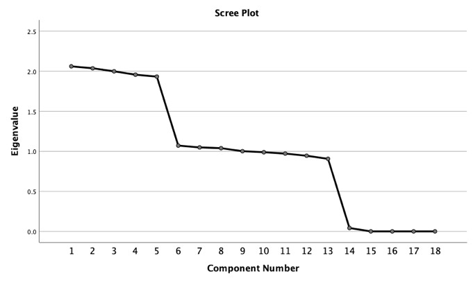
Fig.1. Scree Plot

4. Component Matrix

Table 5 displays the component score Coefficient Matrix. F1 has higher loads for the international expense, F2, F3 and F4 separately have higher loads for the day expense, evening expense and night expense. F5 has higher loads for voice mail.

As a result, we can reliably assume that the call qualities are characterized from F1 to F5. The computation formulae were as follows.

F1=0.998total international minutes + 0.998total international charge

F2= 0.999total day minutes + 0.999total day charge

F3= total evening minutes + total evening charge

F4= total night minutes + total night charges

F5=0.989voice mail plan + 0.989number of voice mail messages

Table 5. Rotated component Matrix

3. Using Logistic regression model of telecom customer churn ptrdiction

3.1. Binary Logistic Regression Model

There are several types of regression analysis, all of which are connected to the number of independent variables as well as the kind of dependent variable [14]. When there is only one independent variable and the dependent variable is numerical, we may either use the basic linear regression model or the multiple linear regression model. The independent variables should be numerical or dichotomous (with values of 0 or 1), therefore if a category variable has two possibilities, these alternatives should be recorded as 0 or 1. If the categorical variable contains three choices (possible answers), it should be placed into the model as two independent variables, one representing the first option and the second representing the second option; in this instance, the interpretation will be a reference to the variable's third option.

In this paper, customer churn prediction will be tackled as a binary classification issue. Companies typically use data mining tools to undertake customer attrition analysis in this situation.

The churn behavior has two values, churning customers are noted as 1, and customers who do not churn are noted as 0.

3.2. Evaluation Criteria

Before making a prediction, the evaluation approach is investigated. The confusion matrix is the most basic technique of measure success and evaluating the model's performance. It displays how frequently each feasible forecast was true or erroneous. The form of confusion matrix as table 6 shows:

Table 6. Confusion Matrix

The abbreviations are presented as TN-True Negatives, FN-False Negatives, FP-False Positives and TP-True Positives. The number of churning customers and non-churning customers separately can be written as:

\( P=TP+FN \)

\( N=TN+FP \)

Recall, precision, accuracy and F1-score also can be derived from the confusion matrix. The recall reflects the reliability of the data, the precision reflects the ability to find all targets to the greatest extent possible. Their formulas are as follows:

\( Recall= \frac{TP}{FP+TP} \)

\( Precision=\frac{TP}{FN+TP} \) \( Accuracy=\frac{TN+TP}{T+P} \)

3.3. Determination of the threshold

Probability classifiers usually have default thresholds t = 0.5, this means every customer whose churning rate is anticipated to be at least 50% will be labelled as such. Because the data is heavily skewed, TP in the confusion matrix will be less useful on its own. If an example with 5% churners, a model that forecasts every entry as a non-churner will have an extremely high TN value, resulting in 95% accuracy while not accurately identifying a single churner. Thus, A stricter threshold will decrease the number of four values and lower the accuracy of the analysis, just like the table 7.

Table 7. Classification when threshold = 0.5

An ideal threshold on which to run a certain model that guarantees a high quantity of acquired TP while not raising FP too much must be found. A broader threshold will identify more data points as churners, resulting in more TP but also more FP. Sometimes P and R indicators are contradictory, so they need to be considered comprehensively. The most common method is F1-measure, F1-measure is Precision and Recall weighted harmonic average, its formula is as follows:

\( F1-score=\frac{2×Precision×Recall}{Precision+Recall} \)

To achieve this goal, we take 10 constant values between 0 and 0.2 as thresholds for a comparison. The result of the comparison is shown below:

Table 8. Comparison of different threshold

Finally, we choose t=0.18 as the threshold. In table 8, the prediction accuracy of the model is demonstrated to be 72.9 per cent, and the F1-Score is 63.45 per cent, this is adequate.

3.4. Analysis of Logistic regression model

Except for Logistic Regression, ROC curve also should be used, ROC curve is combined with two variables: TP rate – sensitivity and TN rate – specificity. If we want to obtain greater sensitivity, a specific ratio of false positives must be considered. Because the data is very skewed, a little increase in the ratio of true positives might result in a significant rise in the quantity of FP. From Figure 2, we can find the curve of international plan voice mail plan, customer service calls, total day minutes and total night minutes are above the reference line, so the area under the curve is greater than 0.5, if the ROC curve is to the upper left corner, the higher the recall rate of the model will be obtained. The point on the ROC curve closest to the upper left corner is the best threshold with the fewest classification errors and the lowest total number of false positive and false negative cases. This means all these variables have impact on customer churn, especially the number of customer service calls.

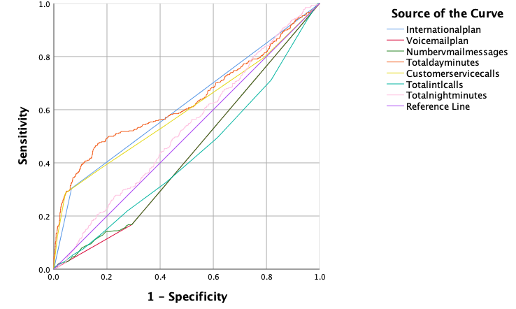
Fig.2. ROC curve of variables

Table 9. Parameter Test

According to the parameter test table 9, we can see the regression coefficient of the account length is 0.001, this is not significant, sig=0.572>0.05, which shows account length does not have an impact on customer churn.

The regression coefficient of the international plan is 2.105, which is significant. Sig =0 < 0.05, this means the international plan has a positive impact on customer churn and demonstrates that consumers who have an international plan will be churned easily because customers will have more choices.

The number of voice mail and customer service calls all have positive impacts on customer churn, the reason is that too many voice mails will make customers turn into e-mails and too many customer service calls demonstrate the quality of calls is bad.

According to the summary analysis, the international plan, the number of voice mail messages and customer service call all have a significant positive impact on customer churn.

On the other hand, the regression coefficient of the total day minutes is -0.013. Sig=0<0.05, this means the total day minutes have a slightly positive impact on customer retention. The reason may be that too much use time will make customers dependent on the products. The regression coefficient of the total night minutes is -0.05, which is not significant. Sig =0 < 0.05, this means the total night minutes still have a positive impact on customer retention and demonstrate customers who have more night calls will not churn. The reason may be that customers enjoy the benefits of discounted night call charges. Voice mail plans and total international calls have a considerable negative influence on customer turnover. The reason may be that voice mail plans will significantly decrease user fees. If a customer makes a lot of international calls, this demonstrates he is satisfied with companies’ service.

The account length, area code, total day calls, total evening minutes, total evening calls, total evening charge, total night calls, total international minutes and total international charge have no effect on customer turnover.

4. Further study

The data of this paper is from three years ago without considering the effect of Covid-19. Because of Covid-19, the telecom market and customer consumption and living habits may be considerably changed. As a result, more recent data will be acquired to increase the model's accuracy and study the effects of Covid-19 on customer churn. For instance, different kinds of isolation policies make people work at home via the internet or mobile phones, whether these conditions will decrease customer churn. Furthermore, the model may be enhanced further by employing the repeated data testing technique.

5. Conclusion

Telecom customer churn is a major concern for telecom firms since it reduces earnings. The logistic regression equation was also confirmed to be true and capable of explaining the causes of churn by the accuracy test. Previous telecom customer churn studies mostly used factor analysis, cluster analysis, and other methodologies, whereas Fisher discriminant analysis and logistic regression analysis research are sparse. This fresh inquiry should resolve the issue.

To maximize the probability of retaining telecom customers, telecom providers should reduce customers' monthly fixed charges and local fees, such as discounts on night calls. Furthermore, telecom executives have recognized the value and significance of improving the service quality of calls and providing preferential policies for phone charges, which have previously been shown to have a positive impact on telecom customer retention.

References

[1]. K. Dahiya and S.Bhatai, "Customer churn analysis in telecom industry," 4th International Conference on Realibility, Infocom Tehnilogies and Optimization(ICRITO), 2015.
[2]. K. Coussement, S. Lessmann, and G. Verstraeten, “A comparative analysis of data preparation algorithms for customer churn prediction: A case study in the telecommunication industry,” DECISION SUPPORT SYSTEMS, vol. 95, pp. 27–36, 2017.
[3]. A. De Caigny, K. Coussement, and K. W. De Bock, “A new hybrid classification algorithm for customer churn prediction based on logistic regression and decision trees,” European journal of operational research, vol. 269, no. 2, pp. 760–772, 2018.
[4]. V. Mahajan, R. Misra, and R. Mahajan, “Review of Data Mining Techniques for Churn Prediction in Telecom,” Journal of information and organizational sciences, vol. 39, no. 2, pp. 183–197, 2015.
[5]. R. Misra, R. Mahajan and V. Mahajan, “Review on factors affecting customer churn in telecom sector,” International journal of data analysis techniques and strategies, vol. 9, no. 2, pp. 122-144, 2017.
[6]. R. Yu, X. An, B. Jin, J. Shi, O. A. Move, and Y. Liu, “Particle classification optimization-based BP network for telecommunication customer churn prediction,” Neural computing & applications, vol. 29, no. 3, pp. 707–720, 2016.
[7]. T. Zhang, S. Moro, and R. F. Ramos, “A Data-Driven Approach to Improve Customer Churn Prediction Based on Telecom Customer Segmentation,” Future internet, vol. 14, no. 3, p. 94, 2022.
[8]. E. A. El Kassem, S. A. Hussein, A. M. Abdelrahman, and F. K. Alsheref, “Customer churn prediction model and identifying features to increase customer retention based on user-generated content,” International journal of advanced computer science & applications, vol. 11, no. 5, pp. 522–531, 2020.
[9]. L. C. Cheng, C.-C. Wu, and C.-Y. Chen, “Behavior Analysis of Customer Churn for a Customer Relationship System: An Empirical Case Study,” global information management, vol. 27, no. 1, pp. 111–127, 2019.Journal of
[10]. Y. Li, B. Hou, Y. Wu, D. Zhao, A. Xie, and P. Zou, “Giant fight: Customer churn prediction in the traditional broadcast industry,” Journal of business research, vol. 131, pp. 630–639, 2021.
[11]. M. Maw, S.-C. Haw, and C.-K. Ho, “Utilizing data sampling techniques on algorithmic fairness for customer churn prediction with data imbalance problems [version 1; peer review: 2 approved with reservations],” F1000 research, vol. 10, p. 988, 2021.
[12]. S. Sun and M. Zhou, “Analysis of farmers’ land transfer willingness and satisfaction based on SPSS analysis of computer software,” Cluster computing, vol. 22, no. Suppl 4, pp. 9123–9131, 2018.
[13]. K. W. De Bock and D. V. den Poel, “An empirical evaluation of rotation-based ensemble classifiers for customer churn prediction,” Expert systems with applications, vol. 38, no. 10, pp. 12293–12301, 2011.
[14]. W. Li and C. Zhou, “Customer churn prediction in telecom using big data analytics,” IOP Conference Series: Materials Science and Engineering, vol. 768, no. 5, p. 52070, 2020.
Cite this article
Wu,S. (2023). Customer Churn Prediction in the Telecommunication Industry. Advances in Economics, Management and Political Sciences,4,41-50.
Data availability
The datasets used and/or analyzed during the current study will be available from the authors upon reasonable request.
Disclaimer/Publisher's Note
The statements, opinions and data contained in all publications are solely those of the individual author(s) and contributor(s) and not of EWA Publishing and/or the editor(s). EWA Publishing and/or the editor(s) disclaim responsibility for any injury to people or property resulting from any ideas, methods, instructions or products referred to in the content.
About volume
Volume title: Proceedings of the 6th International Conference on Economic Management and Green Development (ICEMGD 2022), Part Ⅱ
© 2024 by the author(s). Licensee EWA Publishing, Oxford, UK. This article is an open access article distributed under the terms and
conditions of the Creative Commons Attribution (CC BY) license. Authors who
publish this series agree to the following terms:
1. Authors retain copyright and grant the series right of first publication with the work simultaneously licensed under a Creative Commons
Attribution License that allows others to share the work with an acknowledgment of the work's authorship and initial publication in this
series.
2. Authors are able to enter into separate, additional contractual arrangements for the non-exclusive distribution of the series's published
version of the work (e.g., post it to an institutional repository or publish it in a book), with an acknowledgment of its initial
publication in this series.
3. Authors are permitted and encouraged to post their work online (e.g., in institutional repositories or on their website) prior to and
during the submission process, as it can lead to productive exchanges, as well as earlier and greater citation of published work (See
Open access policy for details).