1. Introduction

Momentum investing is a popular quantitative investment strategy that has gained significant attention in the finance literature over the past few decades. Time series momentum strategy(TSMOS), a subcategory of momentum investing, uses past returns to predict future returns. In this paper, we conduct an empirical analysis of the time series momentum strategy using S&P500 data from 2000 to 2022.

Time series momentum strategy has gained significant attention in the past two decades in the finance literature. It is a quantitative investment strategy that uses past returns to predict future returns. In this paper, we conduct an empirical analysis of the time series momentum strategy using S&P500 data from 2000 to 2022. One of the most influential works in the field of momentum investing is Jegadeesh and Titman. The authors showed that past performance can predict future performance, especially for short-term investments [1]. Building on their work, Moskowitz et al. demonstrated that momentum strategies can generate positive returns in different asset classes, including equities, bonds, currencies, and commodities [2].

Further research has examined the effectiveness of different momentum strategies. Carhart proposed a four-factor model that includes momentum as one of the factors to explain the cross-section of stock returns [3]. Fama and French suggested that the momentum effect is not a distinct factor but rather a manifestation of other fac-tors such as market beta, size, and value [4].

Recent literature has explored more applications of time series momentum strategies. Hutchinson and O'Brien delve into the relationship between time-series momentum and macroeconomic risk. Their study examines how macroeconomic factors impact the performance of momentum strategies and the findings contribute to understanding the underlying dynamics and risk factors associated with momentum investing [5]. Interest rate momentum is explored by Hartley across global yield curves. The study investigates the presence of momentum effects in interest rates in both developed and emerging market countries. The results highlight the pervasiveness of interest rate momentum and its potential implications for fixed income investors [6]. Intraday time-series momentum and investor trading behavior are explored by Onishchenko, Zhao, Kuruppuarachchi, and Roberts, they revealed how institutional and foreign investors' late-informed trading contributes to intraday momentum effects [7]. Examining the performance of time-series momentum strategies across different asset classes, Molyboga, Swedroe, and Qian analyzed data from 78 futures markets, their study highlights the profitability and practical applications of short-term trend-following strategies using daily returns [8]. The study by Molyboga, Qian, and He explores the practical applications of combining carry and time-series momentum strategies, their findings suggest that the combination of carry and time-series momentum can lead to improved risk-adjusted returns and enhance portfolio diversification [9]. Levy and Lopes introduce the concept of dynamic momentum learning and its application in trend-following strategies. The benefits of incorporating dynamic econometric models to adaptively adjust the importance of different look-back periods for individual assets are highlighted [10].

The previous studies, along with others not mentioned here, have significantly contributed to our understanding of time-series momentum in various financial markets. The literature on momentum investing provides valuable insights into the profitability, risk factors, and practical applications of momentum strategies. As momentum remains one of the widely accepted investment approaches, further research in this area will continue to enhance our understanding of its dynamics and implications for investors.

The motivation behind this study is to examine the effectiveness of the time series momentum strategy in generating positive returns in the US stock market, as well as to explore its dynamics and performance using different moving average methods. Specifically, this paper aims to investigate the relationship between time series momentum strategy and idiosyncratic volatility and to evaluate the performance of different moving average methods, such as simple moving average (MA) and exponential moving average (EMA), on the strategy. To achieve these goals, a regression model to estimate the expected returns and volatility of each asset was applied, and then an evaluation of momentum trading strategy based on different moving average was developed. The strategies were evaluated with and without transaction costs.

This paper contributes to the literature by providing empirical evidence on the effectiveness of time series momentum strategy in the US stock market and by exploring the performance of different moving average methods on the strategy. The findings of this study can provide insights for investors and portfolio managers who are interested in implementing momentum strategies in their investment portfolios.

2. Methodology

2.1. Data Description

The data set used in this study was from the S&P500 index, which includes daily closing prices of its constituent stocks. The S&P500 data set is representative of the US stock market and is widely used in academic and industry research, whose content from 2000 to 2022 provides a robust and comprehensive source of data for analyzing the performance of the time series momentum strategy. The data is organized into time series, with each observation corresponding to a trading day from January 1, 2000, to December 31, 2022.

The data cleaning and preprocessing procedures were conducted to ensure data quality, including identifying and correcting missing data, handling outliers, and checking for data consistency.

2.2. The Regression Model

Suppose there is a time series of returns \( {R_{t}} \) . which will be predict using a linear model with past returns at various horizons, or computed with different smoothing methods:

\( R_{t+1}^{e} = α + \sum _{i = 1}^{M}{β_{i}}f_{t}^{i} + {ε_{t+1}} \) (1)

Here, \( {ε_{t+1}} \) is noise and each of the \( M \) factors \( f_{t}^{i} \) can take the form:

\( MA_{t}^{N}=\frac{1}{N}\sum _{s=t-N}^{t}R_{s}^{e} \) (2)

Or

\( EMA_{t}^{N}=\frac{1}{N}\sum _{s=t-N}^{t}{(1-δ)^{t-s}}R_{s}^{e} \) (3)

where \( N \) is the lookback period, \( R_{t+1}^{e} \) is the expected return of the portfolio at time \( t+1 \) , \( α \) is the intercept or constant term in the linear regression model, which represents the expected return of the portfolio when all the factors have a value of zero. \( M \) is the number of factors included in the linear regression model; \( {β_{i}} \) is the coefficient or weights assigned to each of the \( M \) factors, which represents the contribution of each factor to the expected return of the portfolio, where the coefficients are estimated using historical data and are optimized to maximize the predictive power of the linear regression model; \( f_{t}^{i} \) is the values of the \( M \) factors at time \( t \) , which can be represented by the second equation or third equation; \( {ε_{t+1}} \) is the error term or noise in the linear regression model, represents the part of the expected return that is not explained by the factors included in the model. \( MA_{t}^{N} \) is the moving average factor that used in the Momentum Strategy, which calculates the average return of the portfolio over the past \( N \) periods. \( EMA_{t}^{N} \) is the exponential moving average factor that is used in the Momentum Strategy, which calculates the average return of the portfolio over the past \( N \) periods with a decay factor \( ε \) applied to give more weight to recent returns.

The parameters of the model, including the variance \( σ_{ε}^{2} \) of the noise) can be estimated using linear regression (or more sophisticated technique like generalized least squares). Once that is done, the model can be used to make predictions about the next period returns. \( N \) = 24 was set for this model. The training set is set before January 1, 2010, and the test set afterwards.

2.3. Portfolio Evaluation

After fitting the regression model, a momentum trading strategy that generates portfolio weights based on the simple moving average (MA) or exponential moving average (EMA) of asset returns was developed. The MA and EMA of each stock's returns using different window lengths or half-lives were calculated firstly. Based on these averages, the regression coefficients (α and β) for each stock's returns as a function of its MA or EMA, and the portfolio's expected volatility (σ) were estimated. The portfolio weights were then calculated as:

\( portfolio weights=\frac{(moving average*β+α)}{({σ^{2}})} \) (4)

The returns for each portfolio using the weights computed were worked out and then evaluated for different transaction cost coefficients. The performances of equal-weighted portfolios were also calculated for comparison.

3. Results and Discussion

3.1. Model Without Transaction Cost

The numerical results of this model are shown in Table 1. The result indicates a relatively high Sharpe ratio on the training dataset and positive on the testing dataset, which suggests that the strategy is capable of generating significant returns with low risk. However, the maximum drawdown on the test data set is much lower than on the training data, which suggests that the strategy may be overfitting to the training dataset and may not generalise well to unseen data. The skewness and kurtosis values in the result indicate positive for both datasets, means that the returns distribution is positively skewed and leptokurtic. From the below four parameters, the results suggest that the time series momentum trading strategy performs well with the current model, generating significant returns with low risk.

Table 1: Numerical result of the model without transaction cost.

The percentage change of the investment value on both the training and test data set were computed and plotted, which are shown in Figure 1. Based on the trends observed in the two plots, it can be said that the model performs well on both the training and test data sets as the cumulative returns remained stable throughout most of the period. However, there were a few special periods, where the model shows a downward trend, such as during the global financial crisis in 2009, the European sovereign debt crisis in 2012, the US presidential election in 2016, and the COVID-19 pandemic in 2021. These periods of high market volatility had a significant impact on the model's performance. In contrast, during the recovery period of the US stock market in 2008 and 2010, where there were strong upward trends, the momentum strategy performs better as it was designed to capture such trends. Therefore, it can be concluded that the stronger the trend, the better the model's performance, as figure 1 shows.

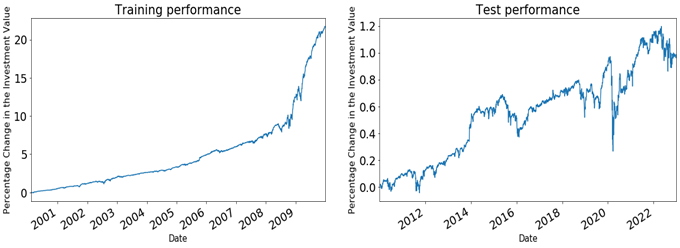
Figure 1: The percentage change of investment value on both training and test data set.

However, it should be noted that the model's performance is better in the training data set than in the test data set. This difference in performance could be attributed to the competitive market environment as this model was more widely known and utilized by investors and the US stock market's relatively low volatility and gradual upward trend, making it harder to capture strong trends. As a result, the returns generated by the model gradually decreased over time.

3.2. Model with Transaction Cost

In this model, three different transaction cost rates were considered, 0.001, 0.005, and 0.01. The Results are shown in Table 2 and 3, and Figure 2, 3 and 4.

Table 2: Numerical result of the model with transaction cost on training data.

Table 3: Numerical result of the model with transaction cost on test data.

We can observe that the model performs well on both datasets in the absence of transaction costs in 3.1, however, the performance is impacted as transaction costs increased. On the training set, considering the relatively low maximum drawdown as well as the positive Sharpe Ratio at all transaction cost rates, it shows the model can generates excess returns with relatively low risk. Moreover, the Sharpe Ratio increases as the transaction cost rate decreases, indicating better performance with lower transaction costs. The skewness is shown relatively high and stable at all transaction cost rates, indicating a right-skewed distribution of returns. The high kurtosis for all transaction cost rates also indicates a sharper distribution than the normal distribution, which however suggests that opportunities to generate large excess returns in this time period were relatively low in the market. On the test set, the impact of transaction cost rate was indicated more obviously. The negative Sharpe Ratio at the 0.01 transaction cost rate shows that it is too high to generate positive returns straightforward. The maximum drawdown also turned to over 7000 when the rate was 0.01 while it was relatively low with lower rates. The low skewness on the 0.01 transaction cost rate indicates a relatively balanced distribution of returns, however the large positive and negative value of skewness on the other two transaction cost rates indicates very right and left skewed distributions of returns. The positively skewed and peaked return distribution suggests that the model is probably taking advantage of trends in the market and profiting from positive momentum. However, considering with the high kurtosis, it indicates again there are not many opportunities to generate large excess returns in the market with high transaction costs.

By checking the graph results - the change of investment value, it is not hard to see that when transaction cost rate is at 0.001, there is little difference in returns before and after costs are added. However, when transaction cost rate increases to 0.005 to 0.01, the difference in returns becomes significant. This indicates that the original model that with-out transaction costs is too idealistic, and transaction costs play a critical role in determining profitability. Furthermore, when the test data was applied to this model, the cumulative returns steadily de-creased. This result is likely because the portfolios constructed by this model were not profitable in the market environment over the last decade, even without transaction costs. Therefore, it highlights again that transaction costs cannot be ignored as they have a significant impact on profitability in this model, and if profits are not high enough to cover the transaction costs, significant losses could occur, as figure 2, 3 and 4 show.

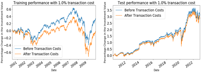
Figure 2: The percentage change of investment value when transaction cost rate = 0.01.

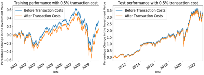
Figure 3: The percentage change of investment value when transaction cost rate = 0.005.

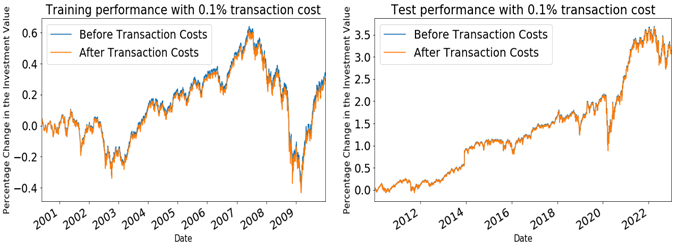
Figure 4: The percentage change of investment value when transaction cost rate = 0.001.

In summary, the model performs well on the training data, generating excess returns with relatively low risk at all transaction cost rates. However, on the test data, varying transaction costs can impact its performance significantly. The better performance at lower transaction cost rates indicates the importance of considering transaction costs in investment strategies. The skewness and kurtosis of the return distribution also vary in different market conditions, therefore, the market conditions, transaction costs and return risks should be considered when implementing the model in actual investments.

3.3. Portfolio Evaluation

The results of portfolio evaluation are shown in Table 4, 5, 6 and 7, where MA and EMA mean simple moving average and exponential moving aver-age, and the followed numbers mean the length of halved life. SR, MD and K mean Sharp Ratio, Maximum Drawdown and Kurtosis respectively; (tr) means on training data and (te) means on test data. The strategies are ranked by the Sharpe Ratio computed on test data.

Table 4: Portfolio evaluation – ranking of strategies when transaction cost rate = 0.

Based on the results, it indicates again that the transaction cost rate has a significant impact on the performance of the trading strategies. In general, the higher the transaction cost rate, the lower the performance of the strategies. This makes sense since transaction costs can eat into the profits of the strategies. For example, when the transaction cost rate is zero, the “MA 1” and “MA 5” strategy has the highest Sharpe ratios in both the training and testing sets, however, when the transaction cost rate is increased to 0.001, the performance of both these strategies deteriorates, and they are outperformed by several other strategies, such as the “Equal Weight” strategy and the “MA 100” strategy, as Table 4, 5, 6 and 7 show.

It seems that the strategies that perform well with low transaction cost rates are also the ones that have relatively high turnover rates, such as the “MA 1” and “MA 5” strategies. On the other hand, the strategies that perform well with high transaction cost rates tend to have lower turnover rates and are more diversified, such as the “Equal Weight” strategy and the “MA 100” strategy.

It is also interesting to note that the performance of some strategies, such as the “MA 2” strategy, deteriorates significantly when the transaction cost rate is increased. This may be because these strategies rely heavily on frequent trading, and the transaction costs can add up quickly and erode their profitability.

Table 5: Portfolio evaluation – ranking of strategies when transaction cost rate = 0.001.

Overall, it is important to take transaction costs into account when evaluating the performance of trading strategies, as they can have a significant impact on the profitability of the strategies. The best strategy will depend on the specific trading scenario, including the expected transaction cost rate, the expected turnover rate, and the expected market conditions.

Table 6: Portfolio evaluation – ranking of strategies when transaction cost rate = 0.005.

Table 7: Portfolio evaluation – ranking of strategies when transaction cost rate = 0.01.

4. Results and Discussion

The results of the study suggest that the time series momentum strategy can be an effective investment strategy for generating positive returns with low risk in the US stock market. The regression model developed in this study shows a high Sharpe ratio on the training dataset and a moderate Sharpe ratio on the testing dataset, indicating that the strategy has the potential to outperform the market. The results also suggest that the momentum effect is present in the US stock market, as the time series momentum strategy generates significant excess returns after controlling for risk factors. The strategy's performance is consistent with previous studies that have shown the effectiveness of momentum strategies in different asset classes and regions. The importance of considering transaction cost and market environment when implementing this model is also emphasized by the results. However, the results also suggest that the strategy was probably overfitting to the training data in this model, as indicated by the high maximum drawdown on the training dataset. Therefore, future studies could explore methods to reduce overfitting, such as using more robust machine learning algorithms or incorporating additional factors into the regression model.

In conclusion, this study provides empirical evidence of the effective-ness of the time series momentum strategy in the US stock market using S&P500 data from 2000 to 2022. The strategy generates positive excess returns with low risk in particular situations, indicating its potential as a profitable investment strategy. The regression model developed in this study provides a framework for implementing the strategy, which involves calculating simple or exponential moving averages of asset returns and estimating the regression coefficients and portfolio weights based on these averages. The strategy can be further optimized by adjusting the window length or half-life of the moving averages and considering transaction costs.

References

[1]. Jegadeesh, N., & Titman, S. (1993). Returns to buying winners and selling losers: Implications for stock market efficiency. The Journal of Finance, 48(1), 65-91.
[2]. Moskowitz, T. J., Ooi, Y. H., & Pedersen, L. H. (2012). Time series momentum. Journal of Financial Economics, 104(2), 228-250.
[3]. Carhart, M. M. (1997). On persistence in mutual fund performance. The Journal of Finance, 52(1), 57-82.
[4]. Fama, E. F., & French, K. R. (2012). Size, value, and momentum in international stock returns. Journal of Financial Economics, 105(3), 457-472.
[5]. Hutchinson, M. C., & O'Brien, J. (2020). Time series momentum and macroeconomic risk. International Review of Financial Analysis, 69, 101469. https://doi.org/10.1016/j.irfa.2020.101469
[6]. Hartley, J. (2020). Interest rate momentum everywhere across global yield curves. SSRN Electronic Journal. https://doi.org/10.2139/ssrn.3542813
[7]. Molyboga, M., Swedroe, L., & Qian, J. (2020). Short-Term Trend: A Jewel Hidden in Daily Returns. The Journal of Portfolio Management, 46(3), 80-93. https://doi.org/10.3905/jpm.2020.1.186
[8]. Onishchenko, O., Zhao, J., Kuruppuarachchi, D., & Roberts, H. (2021). Intraday time-series momentum and investor trading behavior. Journal of Behavioral and Experimental Finance, 31, 100557. https://doi.org/10.1016/j.jbef.2021.100557
[9]. Molyboga, M., Qian, J., & He, C. (2021). Practical applications of carry and time-series momentum: A match made in heaven. The Journal of Alternative Investments. https://doi.org/10.4324/9781315100944-5
[10]. Levy, B. P. C., & Lopes, H. F. (2021). Trend-following strategies via dynamic momentum learning. https://doi.org/10.48550/arXiv.2106.08420
Cite this article
Duan,S. (2023). Performance of Time-series Momentum Strategy: US Evidence. Advances in Economics, Management and Political Sciences,35,45-54.
Data availability
The datasets used and/or analyzed during the current study will be available from the authors upon reasonable request.
Disclaimer/Publisher's Note
The statements, opinions and data contained in all publications are solely those of the individual author(s) and contributor(s) and not of EWA Publishing and/or the editor(s). EWA Publishing and/or the editor(s) disclaim responsibility for any injury to people or property resulting from any ideas, methods, instructions or products referred to in the content.
About volume
Volume title: Proceedings of the 7th International Conference on Economic Management and Green Development
© 2024 by the author(s). Licensee EWA Publishing, Oxford, UK. This article is an open access article distributed under the terms and
conditions of the Creative Commons Attribution (CC BY) license. Authors who
publish this series agree to the following terms:
1. Authors retain copyright and grant the series right of first publication with the work simultaneously licensed under a Creative Commons
Attribution License that allows others to share the work with an acknowledgment of the work's authorship and initial publication in this
series.
2. Authors are able to enter into separate, additional contractual arrangements for the non-exclusive distribution of the series's published
version of the work (e.g., post it to an institutional repository or publish it in a book), with an acknowledgment of its initial
publication in this series.
3. Authors are permitted and encouraged to post their work online (e.g., in institutional repositories or on their website) prior to and
during the submission process, as it can lead to productive exchanges, as well as earlier and greater citation of published work (See
Open access policy for details).