1 Introduction

Consider investors in the financial market, they tend to have a question about how to get an adequate return on their investment. Initially, investors in the market are all following the two basic principles. They all want higher returns from the stock, regardless of various circumstances, preferring more than less. Additionally, the security return will follow the fluctuation of the market, but the investor wants their return on the stock to become more stable and definite. They will find a way to eliminate the uncertainty and correlation among security returns. If the security returns do not correlate with each other. Diversification can help the investor to eliminate the risk. Combining a long list of stocks and bonds is called a portfolio. A portfolio means to combine a long list of stocks and bonds. The amalgamation of different stocks and bonds can protect the investor and increase the opportunity for an investor to succeed. The development of portfolio theory goes through three stages. The first and foremost is the traditional portfolio theory (TPT), as time passed, it goes through the stage of modern portfolio theory (MPT), and post-modern portfolio theory (PMPT).

There are two types of assumptions in MPT. One is the explicit assumption that the returns are all evaluated by a normal distribution. So, it comes out the average returns and standard deviation of returns. The implicit assumption is the theory just ignores the transaction fees and taxes in the market. None of these assumptions are true. However, the efficient market theory is the dominant theory among these assumptions.

A rich array of anomalies that appeared in the market become the burning topic of the current mainstream skepticism of CAPM. The one most closely associated with CAPM is the "Low Beta anomaly" which immediately becomes the most. When people put more effort to observe the pattern of the market. They can notice that higher return α will always correspond to lower β. The asset α produces a negative correlation with asset β. Consequently, it generates an obvious violation in this kind of relationship like lower risk assets correspond to lower returns. Instead, according to CAPM, higher returns always need to bear higher risk. This paper aims to discuss the process of the portfolio theory and CAPM to figure out the problem of low beta anomaly. This paper uses a literature review to analyze the problem of low volatility anomaly.

According to the current complex situation in the industry, Capital Asset Pricing Model (CAPM) still occupies an essential position in the market and stays in the mainstream situation. It can still become a useful tool since it only contains a little flaw. For instance, when people are estimating the asset systematic risk, people tend to use the beta of CAPM to determine the expected rate of return. Considering that people will never know exactly the beta in the asset, so, some scholars advocate using the adjusted beta to replace the beta which is calculated by the regression model. The adjusted beta is 0.67. They use more in portfolio acknowledgment and achievement assessment by maintaining the β which is developed by The Fama–French three-factor model and The Carhart four-factor model.

2 Historical Development of Portfolio Theory

In retrospect, people started to trade with each other around the 1600s. Shares began to appear in the company and the market. However, people came to realize risk at a very backward time. In the 1700s, the market was trying to improve the insurance market system, they began to understand the risk inside the market. Marschak envisioned that future interest from bonds and dividends from stock may be uncertain [1]. Leavens discovered the way to eliminate the risk by diversification [1]. Neumann, Morgenstern, and Savage made a great contribution to the decision-making under risk conditions [1]. By bearing a long-time risk, there were some wise ideas about the CAPM flourishing in society. Markowitz is the founding father of the portfolio theory. He suggested that by using the choice of mean-variance theory to value the assets and proving the basics of mean-variance theory from 1952 to 1959. Markowitz figured out that the problem of inefficient portfolios is the same as the inefficient portfolios [2]. The mean-variance theory was the prototype of the portfolio theory. The portfolio theory was the combination of investments that achieved the highest possible rates of return while taking on the minimum possible risk, in a world of uncertainty. Tobin searched for the interaction between efficient portfolios and monetary assets [1]. A few years after Markowitz's development, Sharpe proposed an idea about the CAPM [1]. It described the link between systematic risk and expected returns. The emergence of Hicks established the mathematical formula for the portfolio theory [1]. Then, Fisher and Lorie studied returns on the stock in 1964. They thought that returns of the stock in the market do not fluctuate over time, which is solid and definite. Until 1968, they discover that the returns of the stock in the market do have a standard deviation. Ibbotson and Sinquefield spent a longer period valuing the equity risk premium [3]. They measured the average return on Standard deviation over 50 years in U.S. and UK. At the same time, Krau, Lee, and Litzenberger provided an alternative theory for the more accurate and realistic result of the return, such as the skewness in the normal distribution [2]. In 1979, there was a new perspective other than people are the all-rational decision-maker in the market proposed by Kahneman and Tversky. Tobin won the Nobel prize for the idea of portfolio selection in 1980. It illustrated how can the changes in the financial market influence the decision-making of households and businesses. In 1996, Barberis et al. proposed that investor is not always rational because they are all human and contains their own emotion and perceptiveness every time. Although, people noticed there are risks involved in the stock. They cannot give a clear definition to distinguish which rate is a good risk and which is a bad risk until Artzner et al. publish the paper in 2000. Artzner then suggested the connection between risk and future wealth. Nevertheless, risk contains different circumstances such as non-satiable or risk-averse other than common risk characteristics. As the idea of risk developed, the idea of the MPT has also achieved a benchmark. The financial theory’s advancement such as the PMPT is largely dependent on the presence of the basic portfolio theory. The major difference between the new and old theories is the expectation of investors. The minimum desired return rate just replaced the average return rate. People who favor using the idea of MPT to determine risk for decades are meeting with the financial crisis in 2008. Investors and Corporate managers were all changed to alternative theories to determine the risk. Instead, people were still discovering and exploring the field of portfolio theory. In 2007, Driessen and Laeven detected international diversification. Maillard et al. unearthed the risk contribution in 2010. The progress of the portfolio theory and CAPM has never ended.

3 Portfolio Theory

3.1 Concept of Risk and Expected Return

Based on the study of investment, the risk might be the probability of an unfortunate event happening, such as the expected return is not as high as the investor expected. The investment risk varies from individual. The reason is that people have their circumstances, and they should find out the right way for their investment. For instance, the emerging situation happens every time such as convene an important meeting. Imagine that you stay up late and need to decide whether to take the subway or take a taxi to the company. Taking a taxi tends to have a higher risk because you might experience traffic congestion while going to the company. On the contrary, the subway can be an unadventurous decision and assure on time. The adventurous person will take the taxi to the company each time. There is also a well-known principle in investment. The more risk a person like to take on, the higher return the person can get.

Return is the fundamental reward of the investment. There are two kinds of return: one is realized return which is the actual money that one has earned; another is expected return which is the expected money you expect to earn. The expected return is based on previous investments to predict future investments.

3.2 Expected Return and Variance for One Security

Take two separate companies to illustrate the portfolio theory. One company is a T-shirt company which sells T-shirts well in summer and bad in winter. The other company is Down jacket company which sells down jackets well in winter and bad in summer. These two companies have the same amount of expected return and profit but in different seasons. The third company sells government bonds which are constant in each of the seasons. The expected profit and return are lower than the first two companies. However, buying bonds in the third company is riskless. From the table, I can calculate the standard deviation of the return of the three companies. Through the calculation, I find out the T-shirt company and down jacket company has higher standard deviation, which means they are more fluctuate. According to the risk, if a person is unwilling to bear the risk, he might prefer to choose a government bond. However, on the other hand, if someone will not bother by the risk and is more adventurous, he might buy one of the bonds in the first two companies.

I study and come to realize that portfolio theory is important in buying bonds. I do the calculation again by changing our strategy for buying 50% of bonds in the T-shirt company and 50% of bonds in the Down jacket company. After I do the simple calculation again, I begin to understand that the portfolio theory gives a high expected return, but a low standard deviation of return. The basic concept of portfolio theory is to combine different investments. This concept will help you to eliminate some of the risks inside of the investment. The diversification effect will benefit people to buy these assets. Assets are risky in the market, so using the portfolio theory can help us to reduce the risk in every investment. Sometimes, I might get a negative expected return by combining the investment, which is called inefficient combinations.

3.3 Expected Return and Variance for Many Securities

The mathematical equation can help work out the rate of return in two securities portfolios. The portion of a portfolio in each asset times the rate of return in each asset can get the total portfolio rate of return.

E[ \( {R_{p}}] \) = \( {x_{1}}× \) E[ \( {R_{1}}]+{x_{2}}× \) E[ \( {R_{2}}] \) (1)

E[ \( {R_{p}}] \) : Expected Return of Portfolio

Before calculating the variance or standard deviation of a portfolio with two securities, I must know the value of the covariance of a portfolio with two securities. The covariance is how much the two assets will move together. If the market is expected covariance is how much the two assets will move together. If the market is expected to be poor, the security will do poorly as well. In addition, returns of the security tend to have a parallel pace with the market. The security will move upward and downward with the market together. The positive covariance illustrates that assets are moving in the same directions. The negative or extremely low covariance demonstrates that assets are moving in opposite directions.

The variance of a portfolio with two securities

\( {{σ_{p}}^{2}} \) = \( {({x_{1}}{σ_{1}})^{2}} \) + \( {({x_{2}}{σ_{2}})^{2}} \) +2( \( {x_{1}})({x_{2}}) {σ_{12}} \) (2)

The standard deviation of a portfolio with two securities

\( {σ_{p}}=\sqrt[]{{({x_{1}}{σ_{1}})^{2}}+{({x_{2}}{σ_{2}})^{2}}+2({x_{1}})({x_{2}}) {σ_{12}}} \) (3)

The crucial idea for the two-bond portfolio’s variance is that I need to add up all possible values with a single value to form the total variance of a portfolio.

Table 2. The variance of a two-bond portfolio

Consequently, I can generalize the portfolio theory from 2 securities to N securities by using the general equation.

Expected mean portfolio return:

E( \( \bar{{R_{p}}} \) )= \( \sum _{i=1}^{N}{x_{i}} \) E( \( \bar{{R_{i}}} \) ) (4)

E( \( \bar{{R_{p}}} \) ): Expected Future Return on the Portfolio invested

E( \( \bar{{R_{i}}} \) ): Expected Future Return on security

Portfolio Risk:

The variance of the portfolio with many securities

Var( \( \bar{{R_{p}}})=\sum _{t=1}^{N}\sum _{s=1}^{N}{x_{t}}{x_{s}} \) cov( \( {R_{s}} \) , \( {R_{t}} \) )(5)

Var( \( \bar{{R_{p}}}): Variance \) , portfolio uncertainty

cov( \( {R_{s}} \) , \( {R_{t}} \) ): Covariance between securities s and t

\( {x_{t}} \) : quantity of security t in the portfolio

\( {x_{s}}: \) quantity of security s in the portfolio

N: quantity of securities in the portfolio

The standard deviation of the portfolio with many securities

\( {σ_{p}}=\sqrt[]{\sum _{t=1}^{N}\sum _{s=1}^{N}{x_{t}}{x_{s}}cov({R_{s}}, {R_{t}})} \) (6)

Table 3. The variance of a portfolio with four securities

After I are picking up all the terms in the matrix, I can get the result of the variance.

\( {{σ_{p}}^{2}}={{x_{1}}^{2}}{{σ_{1}}^{2}}+{{x_{2}}^{2}}{{σ_{2}}^{2}}+{{x_{3}}^{2}}{{σ_{3}}^{2}}+{{x_{4}}^{2}}{{σ_{4}}^{2}}+{2x_{1}}{x_{2}}{σ_{12}}+{2x_{1}}{x_{3}}{σ_{13}}+2{x_{2}}{x_{3}}{σ_{23}}+ 2{x_{1}}{x_{4}}{σ_{14}}+{2x_{2}}{x_{4}}{σ_{24}}+{2x_{3}}{x_{4}}{σ_{34}} \) (7)

4 Capital Asset Pricing Model

4.1 The Hypothesis of the CAPM

There are five basic assumptions in the CAPM.

(1) The market should be highly competitive and the individual investor’s behavior cannot change the market equilibrium price.

(2) The securities holding period is equal for every people who want to invest in the market.

(3) Every people who want to invest in the market are unwilling to undertake the risk, each investor will try to find the most advantageous way to benefit their return according to a different level of risk.

(4) Every people who want to invest in the market must make the same decision in every market situation.

(5) The interest rate is the same for every people who want to lend or borrow money in the market.

4.2 The Efficient Frontier

Imagine I am combining two assets to form the portfolio. It will always generate two lines in the portfolio risk and portfolio return graph. When a different combination is present, it will definitively generate good and bad choices which are a higher return or lower return. People will all tend to invest in the efficient frontier, and nobody will invest in an inefficient portfolio.

In many securities world, people incline to use portfolios for combining different security. All the investors want the efficient frontier to be located in the area with the least amount of risk and greatest return. Consequently, there will be a curve located in the Low Risk& Low Return, Low Risk& High Return, and High Risk& High Return section.

Table 4. Efficient Frontier

Return

Risk

From Figure 1, the dot represents the individual assets. Take two individual assets and put them together to form the portfolio combinations. Finally, it will form the outermost convex hull of all these portfolio combinations. The curve can be deemed to be the upper side and lower side. Since the upper side has a better choice than the lower side, the upper side is called the efficient frontier. Every investor will choose to invest in an efficient area by learning Markowitz’s idea.

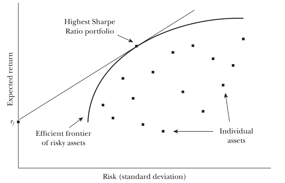
Fig. 1. Efficient Frontier with Many Risky Assets

4.3 Risk-Free Asset

The asset which avoids the risk has 0 percent of variation and invariable returns. While people are investing in the market, they can invest both risk-free assets such as T bills or government bonds and also other assets to form a portfolio frontier. From the portfolio frontier, the turning point in the curve is the point of inflection. The curve above the turning point is the efficient frontier, and the curve below the turning point is an inefficient frontier. The combination of riskless assets and risk assets will form the capital market line (CML). When I calculate the CML, I need to find out both return and risk in riskless assets and risk assets.

Capital Market Line

E[ \( {R_{p}}] \) = \( {r_{f}} \) + \( \frac{E[{R_{p}}]-{r_{f}}}{{σ_{M}}}×{σ_{p}} \) (8)

When I combine the risk-free assets and risk assets, I can get a straight line lie between these two assets. The best line to investigate is the tangent line to the efficient portfolio at only one point, which is called the Capital Market Line or the Capital Allocation Line (CAL). The best portfolio is the amalgamation of risk-free assets and risky assets. It is a mean-variance efficient portfolio. Also, it is the same for everyone, regardless of individual’s wealth and tolerance of risk.

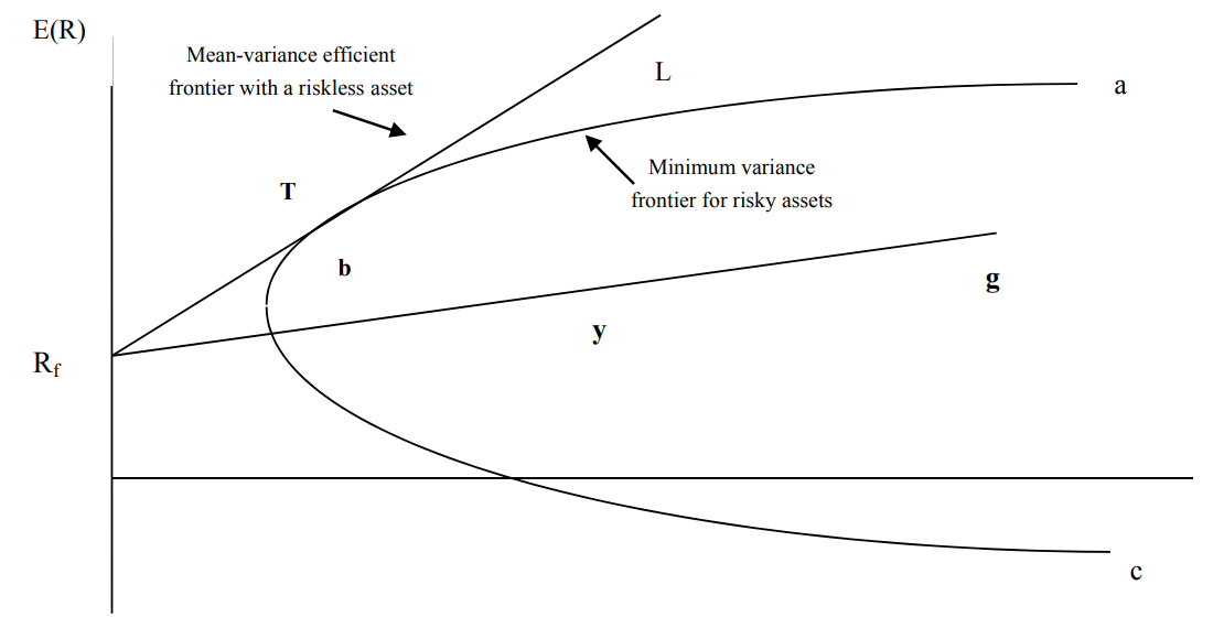
Fig. 2. Investment Opportunities[4]

4.4 Measurement of Risk and Beta Coefficient

Since the risk is varying all the time and is not a specific variable. The variance and standard deviation can be used to consider the risk. The normal distribution curve can also apply in Finance. For example, the return on major corporation common stocks can use the normal distribution to represent. However, diversification can eliminate most of the risk, but not all of the risk. The risk that cannot disappear by combining different assets is called idiosyncratic risk which is unique to the company.

Beta considers the sensitiveness of security to go parallel with the market portfolio. The beta is equal to the ratio of the covariance and variance of the market. There might have some special circumstances where one is the value of the beta in the market and 0 is the value of beta of the risk-free asset.

Beta Coefficient

\( {β_{i}} \) = \( \frac{{σ_{im}}}{{{σ_{m}}^{2}}} \) (9)

\( {σ_{im}}: {Market^{ \prime }}s covariance \)

\( {{σ_{m}}^{2}}: {Market^{ \prime }}s variance \)

Table 5. Betas for different companies

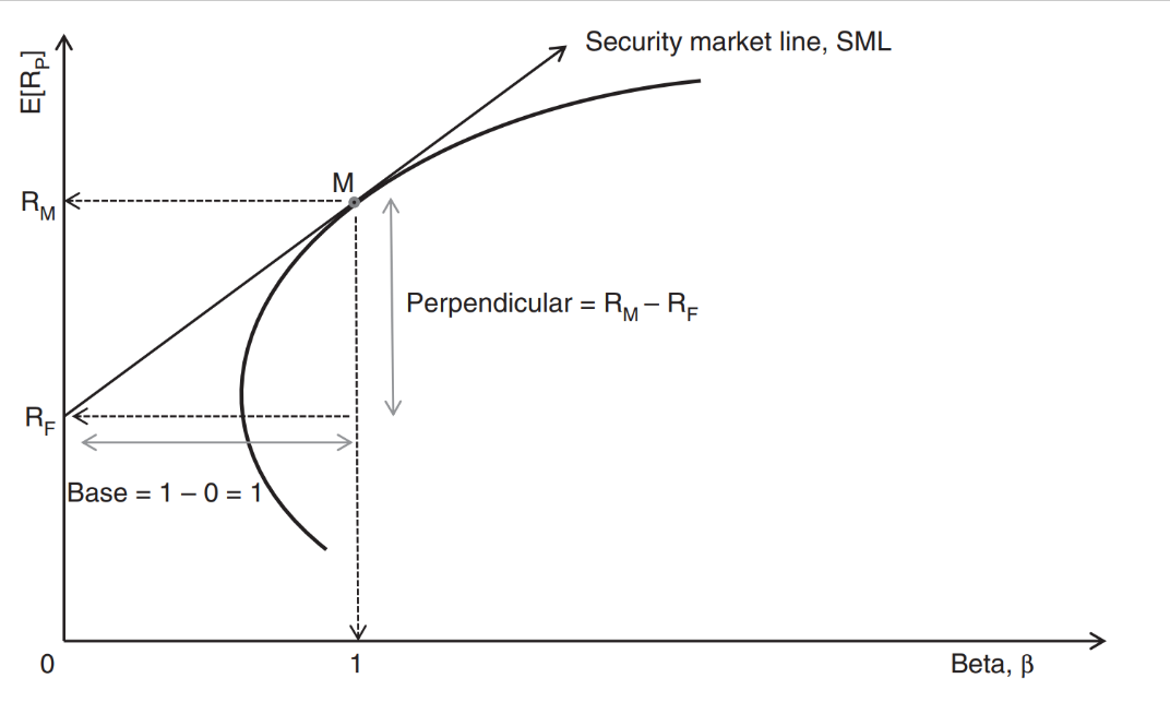
Fig. 3. Security Market Line Model[5]

In theory, the market portfolio should involve all risky securities such as stock, bonds, natural resources, commodities, human capital, etc. When the market is in equilibrium, the security market line (SML) includes all the assets, but when it is not, investors will maintain a higher Sharp ratio and elevate the market portfolio.

The security Market Line

E[ \( {R_{p}}] \) = \( {r_{f}} \) + \( β({r_{m}}-{r_{f}} \) )(10)

4.5 Calculation of the CAPM

The most efficient way to amalgamate all risky assets will produce the best portfolio, which is called a mean-variance efficient portfolio. Further, investors should combine the mean-variance efficient portfolio with the riskless asset to bring up the final CAL. As the previous passage says, the risk is various in diverse people. If the investor is risk-averse, he can invest more money into the riskless asset. On the other hand, if the investor is adventurous, he can invest more money into the mean-variance asset.

The beta in the various portfolio is the ratio of security returns’ covariance and the square of the market returns’ variance.

The beta coefficient in CAPM

\( {β_{i}} \) = \( \frac{Cov({R_{i}}, {R_{M}})}{{σ^{2}}({R_{M}})} \) (11)

The CAPM says the security returns correspond to the beta through the CAPM formula.

\( \bar{{R_{i}}} \) = \( {R_{F}} \) + \( {β_{i}}×(\bar{{R_{M}}}-{R_{F}} \) )(12)

5 Discussion

Through literature review, I found that most of the hypotheses on CAPM are about investors' risk preferences and leverage constraints. From the viewpoint of risk inclination, people who have the opinion about regenerating the profit by “gambling” in their situation are all failing to succeed in their early life. Such investors are not risk-averse, and they might decide on assets with high volatility (high unpredictability) without risk remuneration. The study demonstrates that there is a positive, strong, linear relationship between risk and return. Contrary to the hypothesized association that lower risk will result in higher expected return. Additionally, another viewpoint is leverage constraint, CAPM believes that obtaining leverage financing can help low-risk reluctant over-allocate their assets into risky assets. People should notice and understand this kind of anomaly phenomenon is happening in the market every year when we are using CAPM to calculate the results. However, the generalizability of the results is limited by the natural society or the natural market because of the restriction in finance, so only hazardous and uncertain assets are being invested, resulting in greater current returns and miner future returns. Further research is needed to establish how can the financial market avoiding this kind of anomaly and maintain a stable market.

6 Conclusion

The paper aims to present the MPT. In addition, the paper discusses the revolution of the portfolio theory from TPT to PMPT. From the mean-variance portfolio theory to nowadays generalization of rules in portfolio theory. People tend to understand how a theory can fit into real society. The portfolio theory reflects the relevance between investment and decision-making. The assumption and the correlation between risk and returns help the investor to determine the best way of combining two assets. By combining the risk-free assets and market assets, an investor can eliminate the diversifiable risk.

The CAPM also made a considerable contribution for us to our understanding of how to do the asset pricing. The CAPM illustrates about various investors can reduce an individual’s expected return and price. The beta coefficient in CAPM assesses the receptivity of an individual’s return to the market portfolio. As a result, whether is the portfolio theory or the CAPM, the risk and return in the theory do have some flaws. So, further research on PMPT is kept in research. The PMPT can be more flexible and adjust the flaw of the previous portfolio theory.

References

[1]. Markowitz, Harry M. "The early history of portfolio theory: 1600–1960." Financial analysts journal 55.4 (1999): 5-16.
[2]. Elton, Edwin J., and Martin J. Gruber. "Modern portfolio theory, 1950 to date." Journal of banking & finance 21.11-12 (1997): 1743-1759.
[3]. Perold, André F. "The capital asset pricing model." Journal of economic perspectives 18.3 (2004): 3-24.
[4]. Fama, E. F., & French, K. R. (2004). The Capital Asset Pricing Model: theory and evidence. Journal of Economic Perspectives, 18(3), 25–46.
[5]. Reilly, F., & Brown, K. (2003). Investment analysis portfolio management (7th ed.). Thomson, South-Western.
[6]. What is investment risk?(2020), Barclays Smart Investor [online]. Available from: https://www.barclays.co.uk/smart-investor/new-to-investing/reducing-unnecessary-risk/what-is-investment-risk/ [Accessed 13 March 2022]
[7]. Rau, Raghavendra. Short introduction to corporate finance. Cambridge short introductions to management. Cambridge University Press (2017):42-69
[8]. Markowitz, Harry M. Portfolio selection. Yale university press, 1968:3-8
[9]. Omisore, Iyiola, Munirat Yusuf, and Nwufo Christopher. "The modern portfolio theory as an investment decision tool." Journal of Accounting and Taxation 4.2 (2011): 19-28.
[10]. Rom, Brian M., and Kathleen W. Ferguson. "Post-modern portfolio theory comes of age." Journal of investing 3.3 (1994): 11-17.
[11]. Elbannan, Mona A. "The capital asset pricing model: an overview of the theory." International Journal of Economics and Finance 7.1 (2015): 216-228.
[12]. Bloomberg Guide: Beta, BYU LIBRARY [online]. Available from: https://guides.lib.byu.edu/c.php?g=216390&p=1428678 [Accessed 27 March 2022]
[13]. Constantinides, George M., and Anastasios G. Malliaris. "Portfolio theory." Handbooks in operations research and management science 9 (1995): 1-30.
[14]. Koumou, Gilles Boevi. "Diversification and portfolio theory: a review." Financial Markets and Portfolio Management 34.3 (2020): 267-312.
[15]. Cory Mitchell (2021). William F. Sharpe. Investopedia[online]. Available from: https://www.investopedia.com/terms/w/william-f-sharpe.asp [Accessed 9 April 2022]
[16]. The Investopedia Team (2021). James Tobin. Investopedia[online]. Available from: https://www.investopedia.com/terms/j/james-tobin.asp [Accessed 9 April 2022]
Cite this article
Luo,R. (2023). The Progress of Portfolio Allocation and the Capital Asset Pricing Model. Advances in Economics, Management and Political Sciences,3,374-383.
Data availability
The datasets used and/or analyzed during the current study will be available from the authors upon reasonable request.
Disclaimer/Publisher's Note
The statements, opinions and data contained in all publications are solely those of the individual author(s) and contributor(s) and not of EWA Publishing and/or the editor(s). EWA Publishing and/or the editor(s) disclaim responsibility for any injury to people or property resulting from any ideas, methods, instructions or products referred to in the content.
About volume
Volume title: Proceedings of the 6th International Conference on Economic Management and Green Development (ICEMGD 2022), Part Ⅰ
© 2024 by the author(s). Licensee EWA Publishing, Oxford, UK. This article is an open access article distributed under the terms and
conditions of the Creative Commons Attribution (CC BY) license. Authors who
publish this series agree to the following terms:
1. Authors retain copyright and grant the series right of first publication with the work simultaneously licensed under a Creative Commons
Attribution License that allows others to share the work with an acknowledgment of the work's authorship and initial publication in this
series.
2. Authors are able to enter into separate, additional contractual arrangements for the non-exclusive distribution of the series's published
version of the work (e.g., post it to an institutional repository or publish it in a book), with an acknowledgment of its initial
publication in this series.
3. Authors are permitted and encouraged to post their work online (e.g., in institutional repositories or on their website) prior to and
during the submission process, as it can lead to productive exchanges, as well as earlier and greater citation of published work (See
Open access policy for details).