1. Introduction

The Dickey-Fuller test (DF test) was originally developed by Dickey and Fuller to demonstrate the presence of a unit root. A unit root characteristic of a “non-stationary time series” character theoretically means that the mean and variance of the series are not constant over time. Nyarko mentioned the stationarity of time series data that non-stationary time series data exhibit variant properties with respect to the mean and variance. For time series data that is stationary, the mean and variance will not change over time [1]. This test is a mathematical model that represents the relationship between a time series and its lagged values.

The formula for the DF test as formula 1:

\( {Y_{t}}=p{Y_{t}}-1+{ε_{t}} \) (1)

• \( {Y_{t}} \) is the value of the time series at time t,

• \( p \) is the coefficient on the lagged value of the time series, and

• \( {ε_{t}} \) is an error term.

The null hypothesis is that \( {Y_{t}} \) is not stationary and \( p=1 \) , the error term in the Dickey-Fuller test, is identical and independently distributed [2]. The null hypothesis for the DF test is that \( p=1 \) , which means the time series contains a unit root. However, the alternative hypothesis does not contain a unit root, and p should be smaller than 1. Additionally, if the calculated T statistic in absolute value exceeds the critical value which is usually 0.05, the time series is stationary, but if the calculated T statistic in absolute value is less than the critical value, the time series is non-stationary [3]. The augmented Dickey-Fuller test is an extension of the simple DF test to determine whether financial time series data is stationary or not. This is widespread for statistical tests in econometrics.

The formula for the ADF test as formula 2:

\( Δ{y_{t}}=α+{β_{t}}+γ{y_{t}}-1+δ1Δ{y_{t}}-1+ δ2Δ{y_{t}}-2+… + δpΔ{y_{t}}-p+{Ɛ_{t}} \) (2)

• \( Δ{y_{t}} \) is the first difference of the time series y, ɑ is a constant term,

• \( {β_{t}} \) is a linear trend term,

• \( {y_{t}}-1 \) is the lagged value of \( y \) , \( Δ{y_{t}}-1 \) , \( Δ{y_{t}}-2 \) ,......,

• \( Δ{y_{t}}-p \) are the lagged differences of y up to p lags,

• \( {Ɛ_{t}} \) is the error term.

Compared to the DF test, the ADF test includes additional terms to account for potential trends and serial correlations in the time series. The constant term and linear trend term are helpful to capture any deterministic trends in the time series. Moreover, the lagged value of \( y \) , \( Δ{y_{t}}-1 \) , \( Δ{y_{t}}-2 \) ,......, \( Δ{y_{t}}-p \) can improve the accuracy of the test by reducing type II error when the time series is non-stationary. Similar to the DF test, the null hypothesis is that the time series contains a unit root, which means the series is non-stationary. The alternative hypothesis is the time series is stationary. The series contains a unit root once the series is non-stationary and the first difference is stationary. The ADF test is commonly used to determine the presence of unit roots [4]. For time series data, the ADF test is more flexible and accurate since the financial time series data contains trends or serial correlation.

Since the ADF test can be performed throughout Python, this paper investigates the stationarity of financial time-series data from Nike, and Amazon from 2012 to 2022 by executing the ADF test throughout Python. By using the ADF test to predict stock price and return, The data analysis industry can monitor various listed companies and prevent the crisis caused by the stock market.

2. Methodology

2.1. Data Resource

The monthly stock price for each individual company can be collected from Yahoo Finance. Bitcoin features and prices are freely accessible online. The data to forecasting Bitcoin is collected by using Python 3.6 [5]. Plus, D Shah mentions that the selected financial data of six Indian banks involved in activity between 2004 and 2010 were collected from Yahoo Finance [6]. It illustrates that Yahoo Finance is a trustworthy website to collect data.

After executing the code, there is a data frame for these companies. In this frame, the stock price for each individual company is completely different every day. In other words, financial data is readily available as soon as the data period ends, and today’s stock price is available as soon as the today’s market closes. Fu states that time series can be easily obtained from scientific and financial applications including weekly sales, the price of mutual funds, and stocks. The nature of time series financial data incorporates large data sizes, high dimensionality, and continuous updating [7].

2.2. Process

Once the data is obtained from Yahoo Finance, the author chose the ADF test to test the stationarity of financial time-series data for each company.The augmented Dickey-Fuller test is one of the most useful ways to check the stationarity of time series data. Rhif etc al. state that the wavelet transform (WT) method which decomposes the non-stationary time series into the time frequency domain, is another way to test the stationarity of time series data.

After the test of stationarity, this paper compares the results from the test of stationarity with the plots of stock price and return.

3. Results

3.1. The ADF Test

Based on the Figure 1, the p-values for stock prices are all significantly larger than 0.05, which means it fails to reject the hypothesis. The stock prices of these two companies are non-stationary. However, the p-values for returns are equal to 0, which is smaller than 0.05 (Table 1 and Table 2). In other words, it rejects the null hypothesis. The returns of these two companies are stationary. Shafiee mentions that tomorrow’s stock price is equal to today’s price plus a random shock. The Predictions of non-stationary series do not have any relationship. The movement follows a random work [8].

Table 1: The ADF test for the stock prices.

Table 2: The ADF test for the returns.

3.2. Nike

Figure 1 indicates that the stock price for Nike follows a strong trend, which means the stock price is non-stationary. Figure 2 indicates that the plot of return for Nike does not have a trend, which means the return is stationary. Figure 3 indicates that the autocorrelation of stock price stick to 1, the autocorrelation of return stick to 0.

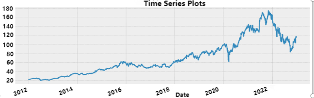
Figure 1: The plot of stock price for Nike.

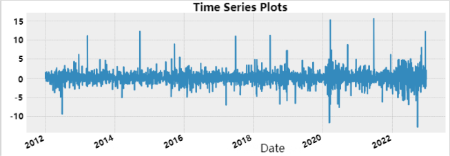
Figure 2: The plot of return for Nike.

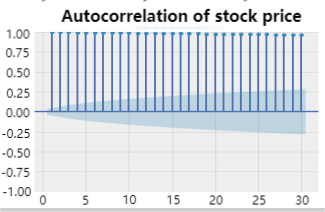
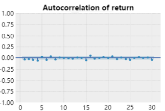
Figure 3: The Autocorrelation of stock price and the autocorrelation of return for Nike.

3.3. Amazon

Figure 4 indicates that the plot of the stock price for Amazon has a strong trend, which means the stock price is non-stationary. Figure 5 indicates that the autocorrelation of stock price sticks to 1, and autocorrelation of return sticks to 0. Figure 6 indicates that the return for Amazon does not have a trend, which means the return is stationary.

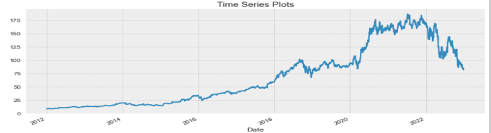
Figure 4: The plot of stock price for Amazon.

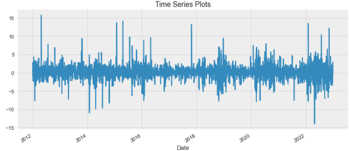
Figure 5: The plot of return for Amazon.

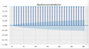
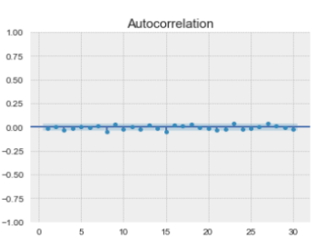
Figure 6: The autocorrelation of stock price for Amazon(left); The autocorrelation of return for Amazon(right).

3.4. Analysis

Based on these graphs, all the plots of stock price are non-stationary since they all have a strong trend, and all the autocorrelation sticks to 1. This is because the stock price is unpredictable. Compared to the plots of stock price, the plots of return do not have a trend at all. All the autocorrelation sticks to 0. So, Nike and Amazon are all market efficient during 2012-2022. The results satisfy that the ADF test, which is used to test the stationarity of financial time-series data, is useful to predict stock price and return for different listed companies since all the p-values for the stock price of these two companies are smaller than 0.05, and all the p-values for the return of these two companies are larger than 0.05. A company could be treated as market efficient once the stock price is non-stationary, and the return is stationary. Furthermore, the ADF test testifies to the characteristics of the plots for stock price and return. Whereas lags refer to the number of lagged differences in the time series being tested that could affect the result of the ADF test. Since the number of lags in the Python code is 30, the test may not fully capture the auto-correlation present in the data. A few lags can lead to a higher probability of a false negative result, which means it fails to reject the null when the series is stationary. Too many lags included may over-correct the auto-correlation, and it rejects the null when the series is non-stationary. Based on the autocorrelation structures and sample sizes, an appropriate number of lags can be picked for the ADF test, and the Akaike Information Criterion (AIC) is one of the various methods to determining the optimal number of lags.

4. Conclusion

This paper mainly introduces the ADF test which is a unit root test to test the stationarity of the financial data. By using the ADF test, it can be concluded that the stock price of Nike and Amazon are non-stationary, and the return of Nike and Amazon are stationary. These two companies are market efficient. The ADF test indicates it is a useful way to predict stock price and return. Since the length of the research date in this paper concentrates on 10 years, the data range may be relatively narrow. Once the range is changed, the null hypothesis of the stock price in the ADF test may be failed to reject, and the null hypothesis of return in the ADF test may be rejected. The data analysis industry may consider that listed companies have potential investment risks.

References

[1]. Lin, L. F., Adjei, B. K., & Nyarko, F. K. The Economic Growth Forecast And A Review Of The Impacts Of Covid-19 On The Ghanaian Economy: Application Of Time Series Analysis And Monte-Carlo Simulation.
[2]. de Carvalho, J. R. P., Assad, E. D., de Oliveira, A. F., & Pinto, H. S. (2014). Annual maximum daily rainfall trends in the Midwest, southeast and southern Brazil in the last 71 years. Weather and Climate Extremes, 5, 7-15.
[3]. Niyimbanira, F. (2013). An overview of methods for testing short-and long-run equilibrium with time series data: Cointegration and error correction mechanism. Mediterranean Journal of Social Sciences, 4(4), 151.
[4]. Glynn, J., Perera, N., & Verma, R. (2007). Unit root tests and structural breaks: A survey with applications.
[5]. Mudassir, M., Bennbaia, S., Unal, D., & Hammoudeh, M. (2020). Time-series forecasting of Bitcoin prices using high-dimensional features: a machine learning approach. Neural computing and applications, 1-15
[6]. Patel, R., & Shah, D. (2016). Mergers and acquisitions-The game of profit and loss: A study of Indian banking sector. Researchers World, 7(3), 92.
[7]. Fu, T. C. (2011). A review on time series data mining. Engineering Applications of Artificial Intelligence, 24(1), 164-181.
[8]. Shafiee, S., & Topal, E. (2010). An overview of global gold market and gold price forecasting. Resources policy, 35(3), 178-189.
Cite this article
Guo,Z. (2023). Research on the Augmented Dickey-Fuller Test for Predicting Stock Prices and Returns. Advances in Economics, Management and Political Sciences,44,101-106.
Data availability
The datasets used and/or analyzed during the current study will be available from the authors upon reasonable request.
Disclaimer/Publisher's Note
The statements, opinions and data contained in all publications are solely those of the individual author(s) and contributor(s) and not of EWA Publishing and/or the editor(s). EWA Publishing and/or the editor(s) disclaim responsibility for any injury to people or property resulting from any ideas, methods, instructions or products referred to in the content.
About volume
Volume title: Proceedings of the 7th International Conference on Economic Management and Green Development
© 2024 by the author(s). Licensee EWA Publishing, Oxford, UK. This article is an open access article distributed under the terms and
conditions of the Creative Commons Attribution (CC BY) license. Authors who
publish this series agree to the following terms:
1. Authors retain copyright and grant the series right of first publication with the work simultaneously licensed under a Creative Commons
Attribution License that allows others to share the work with an acknowledgment of the work's authorship and initial publication in this
series.
2. Authors are able to enter into separate, additional contractual arrangements for the non-exclusive distribution of the series's published
version of the work (e.g., post it to an institutional repository or publish it in a book), with an acknowledgment of its initial
publication in this series.
3. Authors are permitted and encouraged to post their work online (e.g., in institutional repositories or on their website) prior to and
during the submission process, as it can lead to productive exchanges, as well as earlier and greater citation of published work (See
Open access policy for details).